3  Microdata

3.1 Introduction

There is a strong, widespread and increasing demand for NSIs to release Microdata Files (MF), that is, data sets containing for each respondent the score on a number of variables. Microdata files are samples generated from business or social surveys or from the Census or originate from administrative sources. It is in the interest of users to make the microdata as detailed as possible but this interest conflicts with the obligation that NSIs have to protect the confidentiality of the information provided by the respondent.

In Section 1.1 two definitions of disclosure were provided: re-identification disclosure and attribute disclosure. In the microdata setting the re-identification disclosure concept is used as we are releasing information at individual level. When releasing microdata, an NSI must assess the risk of re-identifying statistical units and disclosing confidential information. There are different options available to NSIs for managing these disclosure risks, namely applying statistical disclosure control techniques, restricting access or a combination of the two.

Applying SDC methods leads to a loss of information and statistical content and affects the inferences that users are able to make on the data. The goal for an effective statistical disclosure control strategy is to choose optimum SDC techniques which maximize the utility of the data while minimizing the disclosure risk. On the other hand, the user of protected microdata should obtain most important information on the expected information loss due to SDC process. It enables the assessment of the impact of changes in the original data resulting from the need to protect statistical confidentiality on the quality of the final results of the estimates and analyzes carried out by him/her.

In general, two types of microdata files are released by NSIs, namely public use files (PUF) and research use files (MFR). The disclosure risk in public use files is entirely managed by the design of the file and the application of SDC methods. For research use microdata files SDC methods will be applied in addition to some restrictions on access and use, e.g. under a licence or access agreement, such as those provided by Commission Regulation 831/2202, see Section 2.3. Necessarily the research release files contain more detail than the public use files. The estimated expected information loss should be computed both as total and for each variable separately, if possible.

Some NSIs will also provide access to microdata in datalaboratories/research centres or via remote access/execution. Datalabs allow approved users on-site access to more identifiable microdata. Typically datalab users are legally prohibited from disclosing information and are subject to various stringent controls, e.g. close supervision on-site to protect the security of the data and output checking, to assist with disclosure control. For remote execution researchers are provided with a full description of the microdata. They then send prepared scripts to the NSI who run the analysis, check and return the results. Remote access is a secure on-line facility where the researchers connect to the NSI’s server (via passwords and other security devices) where the data and programs are located. The researchers can submit code for analysis of microdata or in some instances see the files and programs ‘virtually’ on their desktops. Confidentiality protection is by a combination of microdata modification, automatic checks on output requested, manual auditing of output and a contractual agreement. The researcher does not have complete access to the whole data itself; however they may have access to a small amount of unit record information for the purpose of seeing the data structure before carrying out their analysis.

Section 3.2 goes through the whole process of creating a microdata file for external users from the original microdata. The aim of such section is to briefly analyse the different stages of the disclosure process providing references to the relevant sections where each step will be described in more details. Section 3.6 is dedicated to the software. Sections 3.7 and 3.8 provide some examples. Further and more detailed examples can be found in Case studies available on the CASC website (https://research.cbs.nl/casc/handbook.htm#casestudies). Chapter 6 of the current handbook provides more details on different microdata access issues such as research centres, remote access/execution and licensing.

3.2 A roadmap to the release of a microdata file

This section aims at introducing the reader to the process that, starting from the original microdata file as it is produced by survey specialists, ends with the creation of a file for external users. This roadmap will drive you through the six stage process for disclosure, mostly outlined in Section 1.2 i.e.

1. why is confidentiality protection needed;
2. what are the key characteristics and use of the data;
3. disclosure risk (ex ante);
4. disclosure control methods;
5. implementation;
6. assessment of disclosure risk and utility (ex post)

Specifying, for each stage, the peculiarities of microdata release. In Table 3.1 we present an overview of the process.

Stage of disclosure process	Analyses to be carried out / problem to be addressed ⇓ Results expected
1. Why is confidentiality protection needed	Does the data refer to individuals or legal entity? ⇓ We need to protect the statistical unit
2. What are the key characteristics and use of the data	Analysis of the type/structure of the data ⇓ Clear vision of which units need protections
	Analysis of survey methodology ⇓ Type of sampling frame, sample/complete enumeration of strata, further analysis of survey methodology, calibration
	Analysis of NSI objectives ⇓ Type of release (PUF, MFR),dissemination policies, peculiarities of the phenomenon, coherence between multiple releases (PUF and MFR), coherence with released tables and on-line databases, etc.
	Analysis of user needs ⇓ Priorities for variables, type of analysis, etc.
	Analysis of the questionnaire ⇓ List of variables to be removed, variables to be included, some ideas of level of details of structural variables
3. Disclosure risk (ex ante)	Disclosure scenario ⇓ List of identifying variables
	Definition of risk ⇓ Risk measure
	Risk assessment ⇓ If the risk is deemed too high need of disclosure limitation methods
4. Disclosure limitation methods	Analysis of type of data involved, NSI policies and users needs ⇓ Identification of a disclosure limitation method
	Information loss analysis
5. Implementation	Choice of software, parameters and thresholds for different methods
6. assessment of disclosure risk and utility (ex post)	Ex post analysis of disclosure risk and information loss ⇓ In case disclosure risk and/or utility loss is too high, return to step 4 or 5.

Table 3.1: Roadmap to releasing a microdata file

The idea is to identify for each stage of the process choices that have to be made, analyses that need to be done, problems that need to be addressed and methods to be selected. References to the relevant sections where technical topics are discussed in detail will help the beginners in following the process without getting lost in too technical aspects.

We now analyse in turn each of the six stages.

3.2.1 Need of confidentiality protection

The starting point deals with the need of confidentiality protection which is at the base of any release of microdata. If the microdata do not refer to legal entity or individual persons it can be released without confidentiality protection: an example is the amount of rain fall in a region. If microdata pertain only of public variables, in most cases they might be released: the legislation usually treats such data as excluded from statistical confidentiality. However, in general, data refer to individual or enterprises and contains confidential variables (health related data, income, turnover, expenses, etc.) and therefore need to be protected.

3.2.2 Characteristics and uses of microdata

Of course different levels of protection are needed for different type of users. This theme leads us to the second stage of the process i.e. the study of the key uses and characteristics of the data. Here the initial question is whether the microdata file we are going to release is intended for a general public (public use file) or whether it is created for research purpose (research use files). In the latter case the microdata will be released according to predefined procedures and legal binding (see also Section 6.5). The difference in user’s type implies different user’s needs, different disclosure scenarios, different types of analyses we expect to be performed with the released data, different statistics we may intend to preserve and different amount of protection we intend to apply. We now analyse all these issues in terms.

Type and structure of data
Analysis of user needs involves first a study of the survey information content. This should be done together with a survey expert that has a deeper knowledge of the data, phenomenon and possible types of analysis that can be performed on the data.

Typical questions that need to be addressed are:

Which statistical units are involved in the survey? Individuals, enterprises, households, etc. The type of units has a big influence on the risk assessment stage.

Do data present a particular structure? Hierarchical data: students inside schools, graduates inside universities, employees inside an enterprise, individual inside household etc. If this is the case care needs to be taken in checking both levels/types of units involved. E.g., do schools/universities/enterprises need to be protected besides students/graduates/employees?

What type of sampling design has been used? Are there strata (or units of earlier stages in a two- or multistage sampling design) which have been censured? Of course a complete enumeration of a strata (typical in business surveys) implies different and higher risks than a sample. Is two- or multistage sampling used with different types of units in the different stages?

An analysis of the questionnaire is useful to analyse the type of information present in the file: possible identifying variables (of which identifiers and quasi-identifiers), confidential variables and sensitive variables.

Preliminary work on variables
In this stage the setting of objectives from the viewpoint of the NSI and the user are defined. From the NSI side dissemination policies are clarified (e.g. level of dissemination of NACE, geography, etc. or coherence with published tables). From the user point of view a list of priorities in the structural variables of the survey, requests for minimum level of details for such variables and type of analysis to be performed (ratios, weighted totals, regressions, etc).

The characteristics of the phenomenon under study should also be considered as well as the dissemination policy of the Statistical Institute. This is particularly true for example in business data where some NACE classifications may never be released by their own, but always aggregated with others. Such a-priori aggregations generally depend on the economic structure of the country. It is not a sampling or dissemination problem, but rather a feature of the surveyed phenomenon. This will bring to aggregation of categories of some identifying variables deemed too detailed.

The output of this questionnaire analysis should be a preliminary list of variables to be removed and those to be released (because relevant to users need) together with some ideas of their level of details (depending on whether we are releasing a public use file or a research use file). Some examples to clarify these ideas. Variables that shouldn’t be released comprise variables used as internal checks (e.g. some paradata), flags for imputation, variables that were not validated, variables deemed as not useful because containing too many missing values, information on the design stratum from which the unit comes from etc. Obviously also direct identifiers should not be released. The case studies A1 and A2 on microdata release provide examples of such stage.

Categories of identifying variables with too significant identifying power are commonly aggregated into a single category.

This is particularly true when releasing public use files as certain variables when too detailed could retain a level of “sensitivity”. This may not be felt useful and/or appropriate for the general public. For example, in an household expenditure survey we might avoid releasing for the public use file very detailed information on the expenditure for housing (mortgage, rent) or detailed information on the age of the house or its number of rooms (when this is very high) as these might be considered as giving too much information for particular outlying cases.

Geography
Another example is related to the level of geographical details that maybe different for a public use file or a research use file (especially if a data limitation technique is used). This happens because geographical information is a strongly identifying variable. Moreover, the geographical information collected from the respondent may be available in different variables for different purposes (place of birth, place of residence, place of work, place of study, commuting, etc.). All such geographical details need to be coherent/consistent throughout the file. To this end it may be convenient releasing relative information instead of absolute one: for example place of residence can be given at a certain detail (e.g. region) and then the other geographical information (place of work, study etc.) can be released with respect to this one. Examples of possible relative recodings (e.g. with respect to region of residence) are: region of work same as region of residence, different region but same macroregion, different macroregion.

Coherence with published tables
At this initial stage of the analysis information should be collected on what has already been published/what it is going to be released from the microdata set: dissemination plan, which type of tables and what classification/aggregation was used for the variables. This is to avoid different classifications in different release: the geographical breakdown, as well as classification of other variables in the survey (e.g. age, type of work etc.), should be coherent with the published marginals. For example, if a certain classification of the variable age is published in a table the microdata file should use a classification which has compatible break points so that to avoid gaining information by differencing. Release of date of birth is highly discouraged. Also, as far as possible, published totals should be preserved for transparency.

3.2.3 Disclosure risk (ex ante)

Moreover, in case of multiple release of the same survey (e.g. PUF and microdata for research) coherence should be maintained also between different released files in the sense that releasing different files at the same time shouldn’t allow the gaining of more information than for one file alone (see, Trottini et al., 2006). The principles apply also to the release of longitudinal or panel microdata, where the differences between records pertaining to the same case in different waves will reflect ‘events’ that have occurred to that case, as well as the attributes of the individuals.

Once the characteristics and uses of the survey data are clear, it is time to start the real analysis of the disclosure risk in relation to files with originally collected data – ex ante assessment (in one of next subsections we will indicated also on a necessity of making ex post assessment of disclosure risk to verify effciency of used SDC methods). This implies first a definition of possible situations at risk (disclosure scenarios) and second a proper definition of the ‘risk’ in order to quantify the phenomenon (risk assessment).

Disclosure scenario
A disclosure scenario is the definition of realistic assumptions about what an intruder might know about respondents and what information would be available to him to match against the microdata to be released and potentially make an identification and disclosure.

Again different types of releases may require different disclosure scenarios and different definitions of risk. For example the nosy neighbourhood scenario described in Section 3.3.2, possibly with knowledge of the presence of the respondent in the sample (implying that sample uniques are a relevant quantity of interest for risk definition), may be deemed adequate for a public use file. A different trust might be put in a researcher that needs to perform an analysis for research purposes. This implies, as a minimum step, a higher level of acceptable risk and a different scenario the spontaneous identification scenario.

Spontaneous recognition
Spontaneous recognition is possible when the researchers unintentionally recognize some units. For example, when releasing enterprise microdata, it is publicly known that the largest enterprises are generally included in the microdata file because of their significant impact on the studied phenomenon. Moreover, the largest enterprises are also the most identifiable ones as recognisable by all (the largest car producer factory, the national mail delivery enterprise, etc.). Consequently, a spontaneous identification or recognition might occur. A description of different scenarios is presented in Section 3.3.2; examples of spontaneous identification scenarios for MFR are reported in case studies A1 and A2. 

Definition of risk
From the adopted scenario we can extract the list of identifying variables i.e. the variables that may allow the identification of a unit. These will be the basis for defining the risk of disclosure. Intuitively, a unit is at risk of identification when it cannot be confused with several other units. The difficulty is to express this simple concept using sound statistical methodology.

Different approaches are used if the identifying variables are categorical of continuous. In the former case at the basis of the definition is the concept of a ‘key’ (i.e. the combination of categories of the identifying variables): see Section 3.3.1 for a classification of different definitions. Whereas if continuous identifying variables are present in the file a possibility is to use the concept of density: see Ichim (2009) for a detailed analysis of definitions of risk in the case of continuous variables. Of course, the problem is even more complicated when we deal with a mixture of categorical and numerical key variables; for an example of this situation (quite common in enterprise microdata) see case study A1 (Community Innovation Survey). Another solution in this context can be the assessment of disclosure risk based on the (expected) number of units for which a value of the given continuous variable falls into the respectively defined (using established threshold of deviation) neighborhood of a given observation. This approach can be perceived as some variation of \(k\)-anonymity in this case.

Risk assessment
Once a formal definition of risk has been chosen we need to measure/estimate it. There are several possibilities for categorical identifying variables (these are reported in various subsections of Section 3.3) and for a mixture of categorical and continuous identifying variable we have already mentioned Case study A1. The final step of the risk assessment is the definition of a threshold to define when a unit or a file presents an acceptable risk and when, on the contrary, it has to be considered at risk. This threshold depends of course on the type of measure adopted and details on how to choose a threshold are reported in the relevant subsequent sections.

Choice of scenarios and level of acceptable risk are extremely dependent on different cultural situations in different member states, different policies applied by different institutes, different approaches to statistical analysis, different perceived risk. To this end it must be stressed that different countries may have extremely different situation/phenomenon therefore different scenarios and risk methods are indeed necessary.

Currently there is no general agreement on which risk methodology is best although different methods give in general similar answers for the extreme cases. However, as already stated in Section 3.3.1, there is a strong need to further compare and understand differences between available methods. Pros and cons of each method are described in the relevant sections may be used as a guidelines for the most appropriate choice of the risk estimation in different situations. Further advice can be gained by studying of the examples and case studies.

3.2.4 SDC-methods

If the risk assessment stage shows that the disclosure risk is high then the application of statistical disclosure limitation methods is necessary to produce a microdata file for external users.

Masking methods
Microdata protection methods can generate a protected microdata set either by masking original data, i.e. generating a modified version of the original microdata set or by generating synthetic data that preserve some statistical properties of the original data. Synthetic data are still difficult to implement; a description can be found in Section 3.4.7. Masking methods are divided into two categories depending on their effect on the original data (Willenborg and De Waal, 2001): perturbative and non perturbative masking methods.

Perturbative methods either modify the identifying variables or modify the confidential variables before publication. In the former way, unique combinations of scores of identifying variables in the original dataset may disappear and new unique combinations may appear in the perturbed dataset. In this way a user cannot be certain of an identification. Alternatively confidential variables can be modified; in this case even if an identification occurs, the wrong value is associated and disclosure of the original value is avoided (for an example of this case see case study A2). For a description of a variety of perturbative methods see sections 3.4.2, 3.4.4, 3.4.5 and 3.4.6.

Non-perturbative methods do not alter the values of the variables (either identifying or confidential); rather, they produce a reduction of detail in the original dataset. Examples of non-perturbative masking are presented in Section 3.4.3.

The choice between a data reduction and a data perturbation method strongly depends on the policy of an institute and on the type of data/survey to be released. While the policy of an institute is outside of this debate, technical reasons may suggest the use of perturbative methods for the protection of continuous variables (mainly business data). Analysis of information loss should always be part of the selection process. The usual difference between types of release remains valid and it is linked to the difference between users needs. Again the examples and the case studies A1 and A2 may help in clarifying different situations.

User needs and types of protection
From the needs of the users and the types of analyses that could be performed on the data one could gain information for the choice of the type of protection that could be applied to the microdata. Also users could express priorities in the need of maintaining some variables intact (e.g., for business usually NACE is the most important variable, then employees, and so on).

Information loss
For research purposes maybe we could be interested in maintaining the possibility of being able to reproduce the published tables. For a public use file maybe we could avoid, as much as possible, the use of local suppression as this may render data analysis difficult for non sophisticated users. In general, the implementation of perturbative methods should take into account what variables and relationships among them need to be kept from the user point of view. An assessment of information loss caused by the protection methods adopted is highly recommended. A brief description of information loss measures is reported in Section 3.5; examples of how to check in practice the amount of distortion or modification in the protected microdata is presented in case studies A1 and A2.

Finally, every time a data perturbation method is applied attention should be placed at relationships between different types of release (PUF, MFR, tables) so as to avoid as much as possible, different marginal totals from different sources.

An example of the application of this reasoning for the definition of a dissemination strategy can be found, for example, in Trottini et al. (2006).

3.2.5 Implementation

The next stage of the SDC process is the implementation of the whole procedure, choice of software, parameters and levels of acceptable risks.

Documentation is an essential part of any dissemination strategy both for auditing from external authorities and transparency towards users. The former may include description of legal and administrative steps for a risk management policy together with the technical solution applied. The latter is essential for a user to understand what has been changed or limited in the data because of confidentiality constraints. If a data perturbation method has been applied then, for transparency reasons, this should be clearly stated. Information on which statistics have been preserved and which have been modified and some order of magnitude of possible changes should be provided as far as possible. If a data reduction method has been applied with some local suppression then the distribution of such suppressions should be given for a series of different dimensions of interest (distribution by variables, by household size, household type, etc.) and any other statistics that are deemed relevant for the user. The released microdata should be obviously accompanied by all necessary metadata and information on methodologies used at various stage of the survey process (sampling, imputation, validation, etc.) together with information on magnitude of sampling errors, estimation domains etc.

3.2.6 Ex post assessment of disclosure risk and information loss

The last - but, of course, not least - stage of the procedure is the ex post assessment of disclosure risk and computation of the expected information loss due to SDC. The ex post risk assessment (usually made using the same measures as in the case of ex ante assessement, for comparability) allows for confirmation whether the used procedure eliminates or sufficiently reduces the threat of unit identification or not. If not, a modification of used methods (e.g. by changing some tools, modification of parameters, etc.) should be made. This means back to either the step “Disclosure limitation methods” or the step “Implementation”.

An assessment of information loss caused by the applied protection methods is highly recommended. The knowledge of possible loss of information is key for data utility for possible users. If the information loss is too great then the used methods or their parameterization should be changed (coming back to step “Disclosure limitation methods”). One should remain that simultaneously the disclosure risk should be also as small as possible. Thus, these quantities should be harmonized. A detailed description of information loss measures is reported in Section 3.5; examples of how to check in practice the amount of distortion or modification in the protected microdata is presented in case studies A1 and A2.

Of course, the results of computation of discloure risk (both final and indirect, if applicable) and information loss should be saved in the documentation of the whole process. However, whereas the values of measures of disclosure risk are confidential and known only by entitled staff of the data holder, the level of expected information loss should be made available to the user. It is a very important factor influencing the quality of the final analysis results obtained by him/her.

3.3 Risk assessment

3.3.1 Overview

Microdata has many analytical advantages over aggregated data, but also poses more serious disclosure issues because of the many variables that are disseminated in one file. For microdata, disclosure occurs when there is a possibility that an individual can be re-identified by an intruder using information contained in the file, and when on the basis of that, confidential information is obtained. Microdata are released only after taking out directly identifying variables, such as names, addresses, and identity numbers. However, other variables in the microdata can be used as indirect identifying variables. For individual microdata this are variables such as gender, age, occupation, place of residence, country of birth, family structure, etc. and for business microdata variables such as economic activity, number of employees, etc. These (indirect) identifying variables are mainly publicly available variables or variables that are present in public databases such as registers.

If the identifying variables are categorical then the compounding (cross-classification) of these variables defines a key. The disclosure risk is a function of such identifying variables/keys either in the sample alone or in both the sample and the population.

To assess the disclosure risk, we first need to make realistic assumptions about what an intruder might know about respondents and what information will be available to him to match against the microdata and potentially make an identification and disclosure. These assumptions are known as disclosure risk scenarios and more details and examples are provided in the next section of this handbook. Based on the disclosure risk scenario, the identifying variables are determined. The other variables in the file are confidential or sensitive variables and represent the data not to be disclosed. NSIs usually view all non-publicly available variables as confidential/sensitive variables regardless of their specific content, though there can be some variables, e.g. sexual identity, health conditions, income, that can be more sensitive.

In order to undertake a risk assessment of microdata, NSIs might rely on ad-hoc methods, experience and checklists based on assessing the detail and availability of identifying variables. There is a clear need for obtaining quantitative and objective disclosure risk measures for the risk of re-identification in the microdata. For microdata containing censuses or registers, the disclosure risk is known as we have all identifying variables available for the whole population. However, for microdata containing samples the population base is unknown or partially known through marginal distributions. Therefore, probabilistic modelling or heuristics are used to estimate disclosure risk measures at population level, based on the information available in the sample. This section provides an overview of methods and tools that are available in order to estimate quantitative disclosure risk measures.

Intuitively, a unit is at risk if we are able to single it out from the rest. The idea at the base of the definition of risk is a way to measure rareness of a unit either in the sample or in the population.

When the identifying variables are categorical (as it is usually the case in social surveys) the risk is cast in terms of the cells of the contingency table built by cross-tabulating the identifying variables: the keys. Consequently all the records in the same cell have the same value of the risk.

A classification of risk measures
Several definitions of risk have been proposed in the literature; here we focus mainly on those for which tools are available to compute/estimate them easily. We can broadly classify disclosure risk measures into three types: risk measures based on keys in the sample, those based on keys in the population and that make use of statistical models or heuristics to estimate the quantities of interest and those based on the theory of record linkage. Whereas the first two classes are devoted to risk assessment for categorical identifying variables the third one may be used for categorical and continuous variables.

Risk based on keys in the sample
For the first class of risk measures a unit is at risk if its combination of scores on the identifying variables is below a given threshold. The threshold rule used within the software package \(\mu\)‑ARGUS is an example of this class of risk measures.

Risk based on keys in the population
For the second type of approach we are concerned with the risk of a unit as determined by its combination of scores on the identifying variables within the population or its probability of re-identification. The idea then is that a unit is at risk if such quantity is above a given threshold. Because the frequency in the population is generally unknown, it may be estimated through a modelling process. Examples of this reasoning are the individual risk of disclosure based on the Negative Binomial distribution developed by Benedetti and Franconi (1998) and Franconi and Polettini (2004), which is outlined in Section 3.3.5, and the one based on the Poisson distribution and log-linear models developed by Skinner and Holmes (1998) and Elamir and Skinner (2004) which is described in Section 3.3.6 along with current research on other probabilistic methods. Another approach based on keys in the population is the Special Uniques Detection (SUDA) Algorithm developed by Elliot et al. (2002) that uses a heuristic method to estimate the risk; this is outlined in Section 3.3.7.

Risk based on record linkage
When identifying variables are continuous we cannot exploit the concept of rareness of the keys and we transform such concept into rareness in the neighbourhood of the record. A way to measure rareness in the neighbourhood is through record linkage techniques. This third class of disclosure risk is covered in Section 3.3.8.

Section 3.3.2 provides an introduction to disclosure risk scenarios and Section 3.3.3 introduces concepts and notation used throughout this chapter. Sections to 3.3.8 describe different approaches to microdata risk assessment as specified above. However, as microdata risk assessment is a novelty in statistical research there isn’t yet agreement on what method is the best, or at least best under given circumstances. In the following sections we comment on various approaches to risk measures and try to give advice on situations where they could or could not be applied. In any case, it has been recognised that research should be undertaken to evaluate these different approaches to microdata risk assessment, see for example Shlomo and Barton (2006).

The focus of these methods and this section of the handbook is for microdata samples from social surveys. For microdata samples from censuses or registers the disclosure risk is known. Business survey microdata are not typically released due to their disclosive nature (skewed distributions and very high sampling fractions).

In Section 3.7 we make some suggestions on practical implementation and in Section 3.8 we give examples of real data sets and ways in which risk assessment could be carried out.

3.3.2 Disclosure risk scenarios

The definition of a disclosure scenario is a first step towards the development of a strategy for producing a “safe” microdata file (MF). A scenario synthetically describes (i) which is the information potentially available to the intruder, and (ii) how the intruder would use such information to identify an individual i.e. the intruder’s attack means and strategy. Often, defining more than one scenario might be convenient, because different sources of information might be alternatively or simultaneously available to the intruder. Moreover, re-identification risk can be assessed keeping into account different scenarios at the same time.

We refer to the information available to the intruder as an External Archive (EA), where information is provided at individual level, jointly with directly identifying data, such as name, surname, etc. The disclosure scenario is based on the assumption that the EA available to the intruder is an individual microdata archive. That is, for each individual directly identifying variables, and some other variables are available. Some of these further variables are assumed to be available also in the MF that we want to protect. The intruder’s strategy of attack would be to use this overlapping information to match direct identifier to a record in the MF. The matching variables are then the identifying variables.

We consider two different types of re-identification, spontaneous recognition and re-identification via record matching (or linkage) according to the information we assume to be available to the intruder. In the first case we consider that the intruder might rely on personal knowledge about one or a few target individuals, and spontaneously recognize a surveyed individual (Nosy Neighbour scenario). In such a case the External Archive contains one (or a few) records relative to detailed personal information. In the second case, we assume that the intruder (who might be an MF user) has access to a public register and that he or she tries to match the information provided by this EA, with that provided by the MF, in order to identify surveyed units. In such a case, the intruder’s chance of identifying a unit depends on the EA main characteristics, such as completeness, accuracy and data classification. Broadly speaking, we assume that the intruder has a lower chance of correctly identifying an individual when the information provided by the EA is not update, complete, accurate, or is classified according to standards different by those used in the statistical survey.

Moreover, as far as statistical disclosure control is concerned, experts are used to distinguish between social and economic microdata (without loss of generality we can consider respectively individuals and enterprises). In fact, the concept of disclosure risk is mainly based on the idea of rareness with respect to a set of identifying variables. For social survey microdata, because of the characteristics of the population under investigation and the nature of the data collected, identifying variables are mainly (or exclusively) categorical. For much of the information collected on enterprises however the identifying variables often take the form of quantitative variables with asymmetric distributions (Willenborg and de Waal, 2001). Disclosure scenarios are then described according to this statement.

The case study part of the Handbook contains examples of the Nosy Neighbour scenario and the EA scenario for social survey data. The issues involved with hierarchical and longitudinal data are also addressed. Finally, scenarios for business survey data are discussed.

In any case the definition of the scenario is essential as it defines the hypothesis underneath the risk estimation and the subsequent protection of the data.

3.3.3 Concepts and notation

For microdata, disclosure risk measures quantify the risk of re-identification. Individual per record disclosure risk measures are useful for identifying high-risk records and targeting the SDC methods. These individual risk measures can be aggregated to obtain global file level disclosure risk measures. These global risk measures are particularly useful to NSIs for their decision making process on whether the microdata is safe to be released and allows comparisons across different files.

Microdata disclosure
Disclosure in a microdata context means a correct record re-identification operation that is achieved by an intruder when comparing a target individual in a sample with an available list of units (external file) that contains individual identifiers such as name and address plus a set of identifying variables. Re-identification occurs when the unit in the released file and a unit in the external file belong to the same individual in the population. The underlying hypothesis is that the intruder will always try to match a unit in the sample \(s\) to be released and a unit in the external file using the identifying variables only. In addition, it is likely that the intruder will be interested in identifying those sample units that are unique on the identifying variables. A re-identification occurs when, based on a comparison of scores on the identifying variables, a unit \(i^*\) in the external file is selected as matching to a unit \(i\) in the sample and this link is correct and therefore confidential information about the individual is disclosed using the direct identifiers.

To define the disclosure scenario, the following assumptions are made. Most of them are conservative and contribute to the definition of a worst case scenario:

1. a sample \(s\) from a population \(\mathcal{P}\) is to be released, and sampling design weights are available;
2. the external file available to the intruder covers the whole population \(\mathcal{P}\); consequently for each \(i \in s\) the matching unit \(i^*\) does always exist in \(\mathcal{P}\);
3. the external file available to the intruder contains the individual direct identifiers and a set of categorical identifying variables that are also present in the sample;
4. the intruder tries to match a unit \(i\) in the sample with a unit \(i^*\) in the population register by comparing the values of the identifying variables in the two files;
5. the intruder has no extra information other than that contained in the external file;
6. a re-identification occurs when a link between a sample unit \(i\) and a population unit \(i^*\) is established and \(i^*\) is actually the individual of the population from which the sampled unit \(i\) was derived; e.g. the match has to be a correct match before an identification takes place.

Moreover we add the following assumptions:

7. the intruder tries to match all the records in the sample with a record in the external file;
8. the identifying variables agree on correct matches, that is no errors, missing values or time-changes occur in recording the identifying variables in the two microdata file.

Notation
The following notation is introduced here and used throughout the chapter when describing different methods for estimating the disclosure risk of microdata.

Suppose the key has \(K\) cells and each cell \(k = 1, \ldots, K\) is the cross-product of the categories of the identifying variables. In general, we will be looking at a contingency table spanned by the identifying variables in the microdata and not a single vector. The contingency table contains the sample counts and is typically very large and very sparse. Let the population size in cell \(k\) of the key be \(F_k\) and the sample size \(f_k\). Also:

\[ \sum_{k = 1}^{K}F_{k} = N,\quad \sum_{k = 1}^{K}f_{k} = n. \]

Formally the sample and population sizes in the models introduced in Section 3.3.5 and 3.3.6 are random and their expectations are denoted by \(n\) and \(N\) respectively. In practice, the sample and population size are usually replaced by their natural estimators; the actual sample and population sizes, assumed to be known.

Observing the values of the key on individual \(i \in s\) will classify such individual into one cell. We denote by \(k(i)\) the index of the cell into which individual \(i \in s\) is classified based on the values of the key.

According to the concept of re-identification disclosure given above, we define the (base) individual risk of disclosure of unit \(i\) in the sample as its probability of re-identification under the worst case scenario. Therefore the risk \(r_i\) that we get is certainly not smaller than the actual risk, the individual risk is a conservative estimate of the actual risk:

\[ r_{i}=\mathbb{P}\left( i \text{ correctly linked with } i^* \mid s , \mathcal{P} \text{, worst case scenario }\right) \tag{3.1}\]

All of the methods based on keys in the population described in this chapter aim to estimate this individual per-record disclosure risk measure that can be formulated as \(1/F_k\). The population frequencies \(F_k\) are unknown parameters and therefore need to be estimated from the sample. A global file-level disclosure risk measure can be calculated by aggregating the individual disclosure risk measures over the sample:

\[ \tau_{1} = \sum\limits_{k}^{}\frac{1}{F_{k}} \]

An alternative global risk measure can be calculated by aggregating the individual disclosure risk measures over the sample uniques of the cross-classified identifying variables. Since the uniques in the population \(F_k = 1\), are the dominant factor in the disclosure risk measure, we focus our attention on sample uniques \(f_k = 1\):

\[ \tau_{2} = \sum\limits_{k}^{}{I(f_{k} = 1)\frac{1}{F_{k}}} \]

where \(I\) represents an indicator function obtaining the value 1 if \(f_k = 1\) or 0 if not.

Both of these global risk measures can also be presented as rates by dividing by \(n\), the sample size or the number of uniques.

We assume that the \(f_k\) are observed but the \(F_k\) are not observed.

3.3.4 ARGUS threshold rule

The ARGUS threshold rule is based on easily applicable rules and views of safety/unsafety of microdata that is used at Statistics Netherlands. The implementation of these rules was the main reason to start the development of the software package \(\mu\)‑ARGUS.

In a disclosure scenario, keys a combination of identifying variables, are supposed to be used by an intruder to re-identify a respondent. Re-identification of a respondent can occur when this respondent is rare in the population with respect to a certain key value, i.e. a combination of values of identifying variables. Hence, rarity of respondents in the population with respect to certain key values should be avoided. When a respondent appears to be rare in the population with respect to a key value, then disclosure control measures should be taken to protect this respondent against re-identification.

Following the Nosy Neighbour scenario, the aim of the \(\mu\)‑ARGUS threshold rule is to avoid the occurrence of combinations of scores that are rare in the population and not only avoiding population-uniques. To define what is meant by rare the data protector has to choose a threshold value for each key. If a key occurs more often than this threshold the key is considered safe, otherwise the key must be protected because of the risk of re-identification.

The level of the threshold and the number and size of the keys to be inspected depend of course on the level of protection you want to achieve. Public use files require much more protection than microdata files under contract that are only available to researchers under a contract. How this rule is used in practice is given in the example of Section 3.7.

If a key is considered unsafe according to this rule, protection is required. Therefore often global recoding and local suppression are applied. These techniques are described in the sections 3.4.3.2 and 3.4.3.4.

3.3.5 ARGUS individual risk methodology

If a distinction between units rare in the sample from a unit rare in the population wants to be made then an inferential step may be followed. In the initial proposal by Benedetti and Franconi (1998), further developed in Franconi and Polettini (2004) and implemented in \(\mu\)‑ARGUS, the uncertainty on \(F_k\) is accounted for in a Bayesian fashion by introducing the distribution of the population frequencies given the sample frequencies. The individual risk of disclosure is then measured as the (posterior) mean of \(\frac{1}{F_k}\) with respect to the distribution of \(F_k|f_k\):

\[ r_{i} = \mathbb{E} \left( \frac{1}{F_{k}} \mid f_{k} \right) = \sum\limits_{h\geq f_{k}} \frac{1}{h} \mathbb{P} \left(F_{k} = h \mid f_{k} \right). \tag{3.2}\]

where the posterior distribution of \(F_k|f_k\) is negative binomial with success probability \(p_k\) and number of successes \(f_k\). As the risk is a function of \(f_k\) and \(p_k\) its estimate can be obtained by estimating \(p_k\). Benedetti and Franconi (1998) propose to use

\[ {\hat{p}}_{k} = \frac{f_{k}}{\sum\limits_{i:k(i)=k}^{}w_{i}} \tag{3.3}\]

where \(\sum\limits_{i:k(i)=k}^{}w_{i}\) is an estimate of \(F_k\) based on the sampling design weights \(w_i\), possibly calibrated (Deville and Särndal, 1992).

When is it possible to apply the individual risk estimation
The procedure relies on the assumption that the available data are a sample from a larger population. If the sampling weights are not available, or if data represent the whole population, the strategy used to estimate the individual risk is not meaningful.

In the \(\mu\)‑ARGUS manual (see e.g. Hundepool et al., 2014) a fully detailed description of the approach is reported. This brief note is based on Polettini (2004).

Assessing the risk for the whole file
The individual risk provides a measure of risk at the individual level. A global measure of disclosure risk for the whole file can be expressed in terms of the expected number of re-identifications in the file. The expected number of re-identifications is a measure of disclosure that depends on the number of records. For this reason, \(\mu\)‑ARGUS evaluates also the re‑identification rate that is independent of \(n\):

\[ \xi = \frac{1}{n}\sum\limits_{k=1}^{K}{f_{k}r_{k}} \quad . \]

\(\xi\) provides a measure of global risk, i.e. a measure of disclosure risk for the whole file, which does not depend on the sample size and can be used to assess the risk of the file or to compare different types of release; for the mathematical details see Polettini (2004).

The percentage of expected re-identifications, i.e. the value \(\psi=100\cdot\xi\%\) provides an equivalent measure of global risk.

Application of local suppression within the individual risk methodology
After the risk has been estimated, protection takes place. One option in protection is the application of local suppression (see Section 3.4.3.4).

In \(\mu\)‑ARGUS the technique of local suppression, when combined with the individual risk, is applied only to unsafe cells or combinations. Therefore, the user must input a threshold in terms of risk, e.g. probability of re-identification, to classify these as either safe or unsafe. Local suppression is applied to the unsafe individuals, so as to lower their probability of being re‑identified under the given threshold.

In order to select the risk threshold, that represents a level of acceptable risk, i.e. a risk value under which an individual can be considered safe, the re‑identification rate can be used. A release will be considered safe when the expected rate of correct re-identifications is below a level the NSI considers acceptable. As the re-identification rate is cast in terms of the individual risk, a threshold on the re-identification rate can be transformed into a threshold on the individual risk (see below). Under this approach, individuals are at risk because their probability of re-identification contributes a large proportion of expected re-identifications in the file.

In order to reduce the number of local suppressions, the procedure of releasing a safe file considers preliminary steps of protection using techniques such as global recoding (see Section 3.4.3.2). Recoding of selected variables will indeed lower the individual risk and therefore the re-identification rate of the file.

Expert level

Threshold setting using the re-identification rate
Consider the re-identification rate \(\xi\): a key \(k\) contributes to \(\xi\) an amount \(r_kf_k\) of expected re‑identifications. Since units belonging to the same key \(k\) have the same individual risk, keys can be arranged in increasing order of risk \(r_k\). Let the subscript (\(k\)) denotes the \(k\)-th element in this ordering. A threshold \(r^*\) on the individual risk can be set. Consequently, unsafe cells are those for which \(r_{k} \geq r^*\) that can be indexed by \((k) = k^{*} + 1,\ldots,K\). The key \(k^{*}\) is in a one-to-one correspondence to \(r^{*}\). This allows setting an upper bound \(\xi^{*}\) on the re‑identification rate of the released file (after data protection) substituting \(r_kf_k\) with \(r^{*}f_{(k)}\) for each (\(k\)). For the mathematical details see Polettini (2004) and the Argus manual (e.g. Hundepool et al., 2014).

The approach pursued so far can be reversed. Therefore, selecting a threshold \(\tau\) on the re-identification rate \(\xi\) determines a key index \(k^{*}\) which corresponds to a value for \(r^{*}\). Using \(r^{*}\) as a threshold for the individual risk keeps the re‑identification rate \(\xi\) of the released file below \(\tau\). The search of such a \(k^{*}\) is performed by a simple iterative algorithm.

Releasing hierarchical files
A relevant characteristic of social microdata is its inherent hierarchical structure, which allows us to recognise groups of individuals in the file, the most typical case being the household. When defining the re-identification risk, it is important to take into account this dependence among units: indeed re-identification of an individual in the group may affect the probability of disclosure of all its members. So far, implementation of a hierarchical risk has been performed only with reference to households, i.e. a household risk.

Allowing for dependence in estimating the risk enables us to attain a higher level of safety than when merely considering the case of independence.

The household risk
The household risk makes use of the same framework defined for the individual risk. In particular, the concept of re-identification holds with the additional assumption that the intruder attempts a confidentiality breach by re-identification of individuals in households.

The household risk is defined as the probability that at least one individual in the household is re-identified. For a given household \(g\) of size \(|g|\), whose members are labelled \(i_1, \ldots, i_{|g|}\), the household risk is:

\[ r^{h}(g) = \mathbb{P} \left(i_{1} \cup i_{2} \cup \ldots \cup i_{|g|} \text { re-identified } \right) \]

and is the same for all the individuals in household \(g\) and equals \(r_{g}^{h}\).

Threshold setting for the household risk
Since all the individuals in a given household have the same household risk, the expected number of re‑identified records in household \(g\) equals \(|g|r_{g}^{h}\). The re‑identification rate in a hierarchical file can be then defined as \(\xi^{h} = \frac{1}{n}\sum\limits_{g=1}^{G}{|g|r_{g}^{h}}\), where \(G\) is the total number of households in the file. The re‑identification rate can be used to define a threshold \(r^{h^{\ast}}\) on the household risk \(r^{h}\), much in the same way as for the individual risk. For the mathematical details see Polettini (2004) and the Argus manual (e.g. Hundepool et al., 2014).

Note that the household risk \(r_{g}^{h}\) of household \(g\) is computed by the individual risks of its household members. For a given household, it might happen that a household is unsafe (\(r_{g}^{h}\) exceeds the threshold) because just one of its members, \(i\), say, has a high value \(r_{i}\) of the individual risk. To protect the households, the followed approach is therefore to protect individuals in households, first protecting those individuals who contribute most to the household risk. For this reason, inside unsafe households, detection of unsafe individuals is needed. In other words, the threshold on the household risk \(r^{h}\) has to be transformed into a threshold on the individual risk \(r_{i}\). To this aim, it can be noticed that the household risk is bounded by the sum of the individual risks of the members of the household: \(r_{g}^{h} \leq \sum\limits_{j=1}^{|g|}r_{i_{j}}\).

Consider to apply a threshold \(r^{h^{\ast}}\) on the household risk. In order for household \(g\) to be classified safe (i.e. \(r_{g}^{h} < r^{h^{\ast}}\)) it is sufficient that all of its components have individual risk less than \(\delta_{g} = r^{h ^{\ast}}/|g|\).

This is clearly an approach possibly leading to overprotection, as we check whether a bound on the household risk is below a given threshold.

It is important to remark that the threshold \(\delta_g\) just defined depends on the size of the household to which individual \(i\) belongs. This implies that for two individuals that are classified in the same key \(k\) (and therefore have the same individual risk \(r_{k}\)), but belong to different households with different sizes, it might happen that one is classified safe, while the other unsafe (unless the household size is included in the set of identifying variables).

In practice, denoting by \(g(i)\) the household to which record \(i\) belongs, the approach pursued so far consists in turning a threshold \(r^{h^{\ast}}\) on the household risk into a vector of thresholds on the individual risks \(r_{i} = 1,\ldots,n\):

\[ \delta_{g} = \delta_{g(i)} = \frac{r^{h^{\ast}}}{|g(i)|} \quad . \]

Individuals are finally set to unsafe whenever \(r_{i} \geq \delta_{g(i)}\); local suppression is then applied to those records, if requested. Suppression of these records ensures that after protection the household risk is below the threshold \(\delta_{g}\).

Choice of identifying variables in hierarchical files
For household data it is important to include in the identifying variables that are used to estimate the household risks also the available information on the household, such as the number of components or the household type.

Suppose one computes the risk using the household size as the only identifying variable in a household data file, and that such file contains households whose risk is above a fixed threshold. Since information on the number of components in the household cannot be removed from a file with household structure, these records cannot be safely released, and no suppression can make them safe. This permits to check for presence of very peculiar households (usually, the very large ones) that can be easily recognised in the population just by their size and whose main characteristic, namely their size, can be immediately computed from the file. For a discussion on this issue see Polettini (2004).

3.3.6 The Poisson model with log-linear modelling

As defined in Skinner and Elamir (2004), assuming that the \(F_{k}\) are independently Poisson distributed with means \(\left\{\lambda_{k} \right\}\) and assuming a Bernoulli sampling scheme with equal selection probably \(\pi\), then \(f_{k}\) and \(F_{k} - f_{k}\) are independently Poisson distributed as: \(f_{k} \mid \lambda_{k} \sim \operatorname{Pois} \left(\pi\lambda_{k} \right)\) and \(F_{k} - f_{k} \mid \lambda_{k} \sim \operatorname{Pois} \left( ( 1 - \pi ) \lambda_{k} \right)\) . The individual risk measure for a sample unique is defined as \(r_{k} = \mathbb{E}_{\lambda_{k}} \left( \frac{1}{F_{k}} \mid f_{k} = 1 \right)\) which is equal to:

\[ r_{k} = \frac{1}{\lambda_{k} (1 - \pi) } \left[ 1 - e^{ - \lambda_{k} (1 - \pi) } \right] \]

In this approach the parameters \(\left\{ \lambda_{k} \right\}\) are estimated by taking into account the structure and dependencies in the data through log-linear modelling. Assuming that the sample frequencies \(f_{k}\) are independently Poisson distributed with a mean of \(u_{k} = \pi\lambda_{k}\), a log-linear model for the \(u_{k}\) can be expressed as: \(\text{log}(u_{k}) = x_{k}^{'}\beta\) where \(x_{k}\) is a design vector denoting the main effects and interactions of the model for the key variables. Using standard procedures, such as iterative proportional fitting, we obtain the Poisson maximum-likelihood estimates for the vector \(\beta\) and calculate the fitted values: \({\hat{u}}_{k} = \text{exp}(x_{k}^{'}\hat{\beta})\). The estimate for \({\hat{\lambda}}_{k}\) is equal to \(\frac{{\hat{u}}_{k}}{\pi}\) which is substituted for \(\lambda_{k}\) in the above formula for \(r_{k}\). The individual disclosure risk measures can be aggregated to obtain a global (file-level) measure:

\[ {\hat{\tau}}_{2} = \sum\limits_{k \in \text{SU}}^{}{\hat{r_k} =}\sum\limits_{k \in \text{SU}}^{}{\frac{1}{{\hat{\lambda}}_{k}(1 - \pi)}\lbrack 1 - e^{- {\hat{\lambda}}_{k}(1 - \pi)}\rbrack} \]

where \(\text{SU}\) is the set of all sample uniques.

More details on this method are available from Skinner and Shlomo (2005, 2006) and Shlomo and Barton (2006).

Expert level

Skinner and Shlomo (2005, 2006) have developed goodness-of-fit criteria for selecting the most robust log-linear model that will provide accurate estimates for the global disclosure risk measure detailed above. The method begins with a log-linear model where a high test statistic indicates under-fitting (i.e., the disclosure risk measures will be over-estimated). Then a forward search algorithm is employed by gradually adding in higher order interaction terms into the model until the test statistic approaches the level (based on a Normal distribution approximation) where the fit of the log-linear model is accepted.

This method is still under development. At present there is a need to develop clear and user-friendly software to implement the method. However, the Office for National Statistics in the UK has used it to inform microdata release decisions. The method is based on theoretical well-defined disclosure risk measures and goodness of fit criteria which ensure the fit of the log-linear model and the accuracy of the disclosure risk measures. It requires a model search algorithm which takes some computer time and requires intervention.

New methods for probabilistic risk assessment are under development based on a generalized Negative Binomial smoothing model for sample disclosure risk estimation which subsumes both the model used in \(\mu\)‑ARGUS and the Poisson log-linear model above. The method is useful for key variables that are ordinal where local neighbourhoods can be defined for inference on cell \(k\). The Bayesian assumption of \(\lambda_{k} \sim \text{Gamma}(\alpha_{k},\beta_{k})\) is added independently to the Poisson model above which then transforms the marginal distribution to the generalized Negative Binomial Distribution: \[ f_{k} \sim \text{NB}(\alpha_{k},p_{k} = \frac{1}{1 + \text{N}\pi_{k}\beta_{k}}) \] and

\[ F_{k}|f_{k} \sim \text{NB}(\alpha_{k} + f_{k},\rho_{k} = \frac{1 + \text{N}\pi_{k}\beta_{k}}{1 + \text{N}\beta_{k}}) \]

where \(\pi_{k}\) is the sampling fraction. In each local neighbourhood of cell k a smoothing polynomial regression model is carried out to estimate \(\alpha_{k}\) and \(\beta_{k}\), and disclosure risk measures are estimated based on the Negative Binomial Distribution, \({\hat{\tau}}_{2} = \sum_{k \in \text{SU}}^{}{\hat{r_k} =}\sum_{k \in \text{SU}}^{}\frac{{\hat{\rho}}_{k}(1 - {\hat{\rho}}_{k})^{{\hat{\alpha}}_{k}}}{{\hat{\alpha}}_{k}(1 - {\hat{\rho}}_{k})}\) , see: Rinott and Shlomo (2005, 2006).

3.3.7 SUDA

The Special Uniques Detection Algorithm (SUDA) (Elliot et.al., 2005) is a software system (windows application available as freeware under restricted licence) that provides disclosure risk broken down by record, variable, variable value and by interactions of those. It is based on the concept of a “special unique”. A special unique is a record that is a sample unique on a set of variables and that is also unique on a subset of those variables. Empirical work has shown that special uniques are more likely to be population unique than random uniques. Special uniques can be classified according to the size and number of the smallest subset of key variables that defines the record as unique, known as minimal sample uniques (MSU). In the algorithm, all MSUs are found for each record on all possible subsets of the key variables where the maximum size of the subsets m is specified by the user.

Expert level

SUDA grades and orders records within a microdata file according to the level of risk. The method assigns a per record matching probability to a sample unique based on the number and size of minimal uniques. The DIS Measure (Skinner and Elliot, 2000) is the conditional probability of a correct match given a unique match:

\[ p(cm \mid um) = \frac{\sum\limits_{k = 1}^{K} I\left(f_{k} = 1 \right)}{\sum\limits_{k = 1}^{K} F_{k} I \left(f_{k} = 1 \right) } \]

and is estimated by a simple sample-based measure which is approximately unbiased without modelling assumptions. Elliot (2005) describes a heuristic which combines the DIS measure with scores resulting from the algorithm (i.e., SUDA scores). This method known as DIS-SUDA produces estimates of intruder confidence in a match against a given record being correct. This is closely related to the probability that the match is correct and is heuristically linked to the estimate of

\[ \tau_2 = \sum\limits_k{I(f_k=1)\frac{1}{F_k}} \]

The advantage of this method is that it relates to a practical model of data intrusion, and it is possible to compare different values directly. The disadvantages are that it is sensitive to level of the max MSU parameter and is calculated in a heuristic manner. In addition it is difficult to compare disclosure risk across different files. However, the method has been extensively tested and was used successfully for the detection of high-risk records in the UK Sample of Anonymized Records (SAR) drawn from the 2001 Census (Merrett, 2004). The assessment showed that the DIS-SUDA measure calculated from the algorithm provided a good estimate for the individual disclosure risk measure, especially for the case when the number of key variables, \(m = 6\). The algorithm also identifies the variables and value of variables that are contributing most to the disclosure risk of the record.

A new algorithm, SUDA2 has been developed, Elliot et al (2005), that improves SUDA using several methods. The development provides a much faster tool that can handle larger datasets.

3.3.8 Record Linkage

Roughly speaking, record linkage consists of linking each record \(a\) in file \(A\) (protected file) to a record \(b\) in file \(B\) (original file). The pair \((a,b)\) is a match if \(b\) turns out to be the original record corresponding to \(a\).

To apply this method to measure the risk of identity disclosure, it is assumed that an intruder has got an external dataset sharing some (key or outcome) variables with the released protected dataset and containing additionally some identifier variables (e.g. passport number, full name, etc.). The intruder is assumed to try to link the protected dataset with the external dataset using the shared variables. The number of matches gives an estimation of the number of protected records whose respondent can be re-identified by the intruder. Accordingly, disclosure risk is defined as the proportion of matches among the total number of records in \(A\).

The main types of record linkage used to measure identity disclosure in SDC are discussed below. An illustrative example can be found on the CASC-website as one of the case-studies linked to this handbook (see https://research.cbs.nl/casc/handbook.htm#casestudies).

3.3.8.1 Distance-based record linkage

Expert level

Distance-based record linkage consists of linking each record \(a\) in file \(A\) to its nearest record \(b\) in file \(B\). Therefore, this method requires a definition of a distance function for expressing nearness between records. This record-level distance can be constructed from distance functions defined at the level of variables. Construction of record-level distances requires standardizing variables to avoid scaling problems and assigning each variable a weight on the record-level distance.

Distance-based record linkage was first proposed in Pagliuca and Seri (1999) to assess the disclosure risk after microaggregation, see Section 3.4.2.3. Those authors used the Euclidean distance and equal weights for all variables. (Domingo-Ferrer and Torra, 2001) later used distance-based record linkage for evaluating other masking methods as well; in their empirical work, distance-based record linkage outperforms probabilistic record linkage (described below). Recently, (Torra and Miyamoto, 2004) have shown that method-specific distance functions might be defined to increase the proportion of matches for particular SDC methods.

The record linkage algorithm introduced in (Bacher, Brand and Bender, 2002) is similar in spirit to distance-based record linkage. This is so because it is based on cluster analysis and, therefore, links records that are near to each other.

The main advantages of using distances for record linkage are simplicity for the implementer and intuitiveness for the user. Another strong point is that subjective information (about individuals or variables) can be included in the re-identification process by properly modifying distances. In fact, the next version of the \(\mu\)‑ARGUS microdata protection package (e.g. Hundepool et al., 2014) will incorporate distance-based record linkage as a disclosure risk assessment method.

The main difficulty of distance-based record linkage consists of coming up with appropriate distances for the variables under consideration. For one thing, the weight of each variable must be decided and this decision is often not obvious. Choosing a suitable distance is also especially thorny in the cases of categorical variables and of masking methods such as local recoding where the masked file contains new labels with respect to the original dataset.

3.3.8.2 Probabilistic record linkage

Expert level

Like distance-based record linkage, probabilistic record linkage aims at linking pairs of records \((a,b)\) in datasets \(A\) and \(B\), respectively. For each pair, an index is computed. Then, two thresholds \(LT\) and \(NLT\) in the index range are used to label the pair as linked, clerical or non-linked pair: if the index is above \(LT\), the pair is linked; if it is below \(NLT\), the pair is non-linked; a clerical pair is one that cannot be automatically classified as linked or non-linked and requires human inspection. When independence between variables is assumed, the index can be computed from the following conditional probabilities for each variable: the probability \(\mathbb{P}\left( 1\mid M \right)\) of coincidence between the values of the variable in two records \(a\) and \(b\) given that these records are a real match, and the probability \(\mathbb{P}\left( 0\mid U \right)\)of non-coincidence between the values of the variable given that \(a\) and \(b\) are a real unmatch.

Like in the previous section, disclosure risk is defined as the number of matches (linked pairs that are correctly linked) over the number of records in file \(A\).

To use probabilistic record linkage in an effective way, we need to set the thresholds \(LT\) and \(NLT\) and estimate the conditional probabilities \(\mathbb{P}\left( 1 \mid M \right)\) and \(\mathbb{P}\left( 0 \mid U \right)\) used in the computation of the indices. In plain words, thresholds are computed from: (i) the probability \(\mathbb{P}\left( \text{LP} \mid U \right)\) of linking a pair that is an unmatched pair (a false positive or false linkage) and (ii) the probability \(\mathbb{P}\left( \text{NP} \mid M \right)\)of not linking a pair that is a match (a false negative or false unlinkage). Conditional probabilities \(\mathbb{P}\left( 1 \mid M \right)\) and \(\mathbb{P}\left( 0 \mid U \right)\) are usually estimated using the EM algorithm (Dempster, Laird and Rubin 1977).

Original descriptions of this kind of record linkage can be found in Fellegi and Sunter (1969) and Jaro (1989). Torra and Domingo-Ferrer (2003) describe the method in detail (with examples) and Winkler (1993) presents a review of the state of the art on probabilistic record linkage. In particular, this latter paper includes a discussion concerning non-independent variables. A (hierarchical) graphical model has recently been proposed (Ravikumar and Cohen, 2004) that compares favourably with previous approaches.

Probabilistic record linkage methods are less simple than distance-based ones. However, they do not require rescaling or weighting of variables. The user only needs to provide two probabilities as input: the maximum acceptable probability \(\mathbb{P}\left( \text{LP} \mid U \right)\) of false positive and the maximum acceptable probability \(\mathbb{P}\left( \text{NP} \mid M \right)\) of false negative.

3.3.8.3 Other record linkage methods

Expert level

Recently, the use of other record linkage methods has also been considered for disclosure risk assessment. While in the previous record linkage methods it is assumed that the two files to be linked share a set of variables, other methods have been developed where this constraint is relaxed. Under appropriate conditions, (Torra, 2004) shows that re-identification is still possible when files do not share any variables. Domingo-Ferrer and Torra (2003) propose the use of such methods for disclosure risk assessment.

3.3.9 References

Bacher J., Brand R., and Bender S. (2002), Re-identifying register data by survey data using cluster analysis: an empirical study. International Journal of Uncertainty, Fuzziness and Knowledge Based Systems, 10(5):589–607, 2002.

Benedetti, R. and Franconi, L. (1998). Statistical and technological solutions for controlled data dissemination, Pre-proceedings of New Techniques and Technologies for Statistics, 1, 225-232.

Coppola, L. and Seri, G. (2005). Confidentiality aspects of household panel survey: the case study of Italian sample from EU-SILC. Monographs of official statistics – Proceedings of the Work session on statistical data confidentiality – Geneve 9-11 November 2005, 175-180.

Cox, L.H. (1995). Protecting confidentiality in business surveys. Business Survey Methods, Cox, B.G., Binder, D.A., Chinnappa, B.N., Christianson, A., Colledge, M.J. e Kott, P.S. (Eds.), New-York: Wiley, 443‑476.

Dempster A. P., Laird N. M., and Rubin D. B. (1977), Maximum likelihood from incomplete data via the em algorithm. Journal of the Royal Statistical Society, 39:1–38, 1977.

Deville, J.C. and Särndal, C.E. (1992). Calibration estimators in survey sampling, Journal of the American Statistical Association 87, 367–382.

Domingo-Ferrer J., and Torra, V. (2001), A quantitative comparison of disclosure control methods for microdata. In P. Doyle, J. I. Lane, J. J. M. Theeuwes, and L. Zayatz, editors, Confidentiality, Disclosure and Data Access: Theory and Practical Applications for Statistical Agencies, pages 111–134, Amsterdam, 2001. North-Holland. https://crises-deim.urv.cat/webCrises/publications/bcpi/cliatpasa01Aquantitative.pdf.

Domingo-Ferrer, J., and Torra, V. (2003), Disclosure risk assessment in statistical microdata protection via advanced record linkage. Statistics and Computing, 13:343–354.

Elamir, E., Skinner, C. (2004) Record-level Measures of Disclosure Risk for Survey Microdata, Journal of Official Statistics, Vol. 22, No. 3, 2006, pp. 525–539. See also: Southampton Statistical Sciences Research Institute, University of Southampton, methodology working paper:
https://eprints.soton.ac.uk/8175/

Elliot, M. J., (2000). DIS: A new approach to the Measurement of Statistical Disclosure Risk. International Journal of Risk Management 2(4), pp 39-48.

Elliot, M. J., Manning, A. M.& Ford, R. W. (2002). 'A Computational Algorithm for Handling the Special Uniques Problem'. International Journal of Uncertainty, Fuzziness and Knowledge Based Systems 5(10), pp 493-509.

Elliot, M. J., Manning, A., Mayes, K., Gurd, J. & Bane, M. (2005). ’SUDA: A Program for Detecting Special Uniques’. Proceedings of the UNECE/Eurostat work session on statistical data confidentiality, Geneva, November 2005

Elliot, M. J., Skinner, C. J., and Dale, A. (1998). 'Special Uniques, Random Uniques, and Sticky Populations: Some Counterintuitive Effects of Geographical Detail on Disclosure Risk'. Research in Official Statistics 1(2), pp 53-67.

Fellegi, I. P., and Sunter, A.B. (1969), A theory for record linkage. Journal of the American Statistical Association, 64(328):1183–1210.

Franconi, L. and Polettini, S. (2004). Individual risk estimation in \(\mu\)-ARGUS: a review. In: Domingo-Ferrer, J. (Ed.), Privacy in Statistical Databases. Lecture Notes in Computer Science. Springer, 262‑272

Franconi, L. and Seri, G. (2000). Microdata Protection at the Italian National Statistical Insititute (Istat): A User Perspective. Of Significance Journal of the Association of Public Data Users – Volume 2 Number 1 2000, page. 57-64.

Hundepool, A., Van de Wetering, A., Ramaswamy, R., Franconi, L., Capobianchi, A., de Wolf, P.P., Domingo-Ferrer, J., Torra, V., Brand, R., and Giessing, S. (2014), \(\mu\)-ARGUS version 5.1 Software and User’s Manual. Statistics Netherlands, Voorburg NL, 2014. https://research.cbs.nl/casc/Software/MUmanual5.1.3.pdf.

Jackson, P., Longhurst, J. (2005), Providing access to data and making microdata safe, experiences of the ONS, proceedings of the UNECE/Eurostat work session on statistical data confidentiality, Geneva, November 2005

Jaro, M.A. (1989), Advances in record-linkage methodology as applied to matching the 1985 census of tampa, florida. Journal of the American Statistical Association, 84(406):414–420.

Pagliuca, D. and Seri, G. (1999), Some results of individual ranking method on the system of enterprise accounts annual survey, Esprit SDC Project, Deliverable MI-3/D2.

Polettini, S. and Seri, G (2004). Revision of “Guidelines for the protection of social microdata using the individual risk methodology”. Deliverable 1.2-D3, available at CASC web site.

Ravikumar, P., and Cohen, W.W. (2004),. A hierarchical graphical model for record linkage. In UAI 2004, USA, 2004. Association for Uncertainty in Artificial Intelligence.

Rinott, Y. ,Shlomo, N (2006) A Generalized Negative Binomial Smoothing Model for Sample Disclosure Risk Estimation ,. PSD'2006 Privacy in Statistical Databases, Springer LNCS proceedings, to appear.

Rinott, Y., Shlomo, N. (forthcoming) A Smoothing Model for Sample Disclosure Risk Estimation, Volume in memory of Yehuda Vardi in the IMS Lecture Notes Monograph Series.

Shlomo, N. (2006), Review of statistical disclosure control methods for census frequency tables, ONS Survey Methodology Bulletin.

Shlomo, N., Barton, J. (2006) Comparison of Methods for Estimating Disclosure Risk Measures for Microdata at the UK Office for National Statistics, PSD'2006 Privacy in Statistical Databases Conference, CD Proceedings, to appear

Skinner, C., Shlomo, N. (2005), Assessing disclosure risk in microdata using record-level measures, proceedings of the UNECE/Eurostat work session on statistical data confidentiality, Geneva, November 2005

Skinner, C.J., Shlomo, N. (2006) Assessing Identification Risk in Survey Microdata Using Log-linear Models, Journal of the American Statistical Association, 103 (483). pp. 989-1001. See also: http://eprints.lse.ac.uk/39112/1/Assessing_Identification_Risk_in_Survey_Microdata%28lsero%29.pdf.

Skinner, C., Holmes, D. (1998), Estimating the re-identification risk per record in microdata, JOS, Vol.14.

Torra, V. (2004), Owa operators in data modeling and re-identification. IEEE Trans. on Fuzzy Systems, vol. 12, no. 5, pp. 652-660.

Torra V., and Domingo-Ferrer J. (2003). Record linkage methods for multidatabase data mining. In V. Torra, editor, Information Fusion in Data Mining, pages 101–132, Germany, Springer.

Torra, V., and Miyamoto, S. (2004),. Evaluating fuzzy clustering algorithms for microdata protection. In J. Domingo-Ferrer and V. Torra, editors, Privacy in Statistical Databases, volume 3050 of LNCS, pages 175–186, Berlin Heidelberg. Springer.

Willenborg, L. and De Waal, T. (1996). Statistical Disclosure Control in Practice. Lecture Notes in Statistics, 111, New-York: Springer Verlag.

Willenborg, L. and De Waal, T. (2001). Elements of statistical disclosure control. Lecture Notes in Statistics, 115, New York: Springer-Verlag.

Winkler, W. E. (1993),. Matching and record linkage. Technical Report RR93/08, Statistical Research Division, U. S. Bureau of the Census (USA), 1993.

3.4 Microdata protection methods

3.4.1 Overview of concepts and methods

In this section we explain the basic concepts and methods related to microdata protection. Sections 3.4.2, 3.4.3, 3.4.4 and 3.4.5 give in-depth descriptions of some particularly complex methods: microaggregation, rank swapping, additive noise and synthetic data (the first two implemented in \(\mu\)‑ARGUS).

A microdata set \(\mathbf{X}\) can be viewed as a file with \(n\) records, where each record contains \(m\) variables on an individual respondent. The variables can be classified in four categories which are not necessarily disjoint:

• Identifiers. These are variables that unambiguously identify the respondent. Examples are the passport number, social security number, etc.
• Quasi-identifiers or key variables. These are variables which identify the respondent with some degree of ambiguity. (Nonetheless, a combination of quasi-identifiers may provide unambiguous identification.) Examples are name, address, gender, age, telephone number, etc.
• Confidential outcome variables. These are variables which contain sensitive information on the respondent. Examples are salary, religion, political affiliation, health condition, etc.
• Non-confidential outcome variables. Those variables which do not fall in any of the categories above.

The purpose of SDC is to prevent confidential information from being linked to specific respondents. Therefore, we will assume in what follows that original microdata sets to be protected have been pre-processed so as to remove identifiers and quasi-identifiers with low ambiguity (such as name).

The purpose of microdata SDC mentioned in the previous section can be stated more formally by saying that, given an original microdata set \(\mathbf{X}\), the goal is to release a protected microdata set \(\mathbf{X}'\) in such a way that:

1. Disclosure risk (i.e. the risk that a user or an intruder can use \(\mathbf{X}'\) to determine confidential variables on a specific individual among those in \(\mathbf{X}\)) is low.
2. User analyses (regressions, means, etc.) on \(\mathbf{X}'\) and on \(\mathbf{X}\) yield the same or at least similar results.

Microdata protection methods can generate the protected microdata set \(\mathbf{X}'\)

• either by masking original data, i.e. generating \(\mathbf{X}'\) a modified version of the original microdata set \(\mathbf{X}\);
• or by generating synthetic data \(\mathbf{X}'\) that preserve some statistical properties of the original data \(\mathbf{X}\).

Masking methods can in turn be divided in two categories depending on their effect on the original data (Willenborg and DeWaal, 2001):

• Perturbative masking. The microdata set is distorted before publication. In this way, unique combinations of scores in the original dataset may disappear and new unique combinations may appear in the perturbed dataset; such confusion is beneficial for preserving statistical confidentiality. The perturbation method used should be such that statistics computed on the perturbed dataset do not differ significantly from the statistics that would be obtained on the original dataset.
• Non-perturbative masking. Non-perturbative methods do not alter data; rather, they produce partial suppressions or reductions of detail in the original dataset. Global recoding, local suppression and sampling are examples of non-perturbative masking.

At a first glance, synthetic data seem to have the philosophical advantage of circumventing the re-identification problem: since published records are invented and do not derive from any original record, some authors claim that no individual having supplied original data can complain from having been re-identified. At a closer look, some authors (e.g., Winkler, 2004 and Reiter, 2005) claim that even synthetic data might contain some records that allow for re-identification of confidential information. In short, synthetic data overfitted to original data might lead to disclosure just as original data would. On the other hand, a clear problem of synthetic data is data utility: only the statistical properties explicitly selected by the data protector are preserved, which leads to the question whether the data protector should not directly publish the statistics he wants preserved rather than a synthetic microdata set.

So far in this section, we have classified microdata protection methods by their operating principle. If we consider the type of data on which they can be used, a different dichotomic classification applies:

• Continuous data. A variable is considered continuous if it is numerical and arithmetic operations can be performed with it. Examples are income and age. Note that a numerical variable does not necessarily have an infinite range, as is the case for age. When designing methods to protect continuous data, one has the advantage that arithmetic operations are possible, and the drawback that every combination of numerical values in the original dataset is likely to be unique, which leads to disclosure if no action is taken.
• Categorical data. A variable is considered categorical when it takes values over a finite set and standard arithmetic operations do not make sense. Ordinal scales and nominal scales can be distinguished among categorical variables. In ordinal scales the order between values is relevant, whereas in nominal scales it is not. In the former case, max and min operations are meaningful while in the latter case only pairwise comparison is possible. The instruction level is an example of ordinal variable, whereas eye colour is an example of nominal variable. In fact, all quasi-identifiers in a microdata set are normally categorical nominal. When designing methods to protect categorical data, the inability to perform arithmetic operations is certainly inconvenient, but the finiteness of the value range is one property that can be successfully exploited.

3.4.2 Perturbative masking

Perturbative statistical disclosure control (SDC) methods allow for the release of the entire microdata set, although perturbed values rather than exact values are released. Not all perturbative methods are designed for continuous data; this distinction is addressed further below for each method.

Most perturbative methods reviewed below (including noise addition, rank swapping, microaggregation and post-randomization) are special cases of matrix masking. If the original microdata set is \(\mathbf{X}\), then the masked microdata set \(\mathbf{X}'\) is computed as

\[ \mathbf{X}'=\mathbf{A}\mathbf{X}\mathbf{B} + \mathbf{C} \]

where \(\mathbf{A}\) is a record-transforming mask, \(\mathbf{B}\) is a variable-transforming mask and \(\mathbf{C}\) is a displacing mask or noise (Duncan and Pearson, 1991).

Table 3.2 lists the perturbative methods described below. For each method, the table indicates whether it is suitable for continuous and/or categorical data.

Method	Continuous data	Categorical data
Noise addition	X
Microaggregation	X	(X)
Rank swapping	X	X
Rounding	X
Resampling	X
PRAM		X
MASSC		X

Table 3.2: Perturbative methods vs. data types. “X” denotes applicable and “(X)” denotes applicable with some adaptation.

3.4.2.1 Noise addition

The main noise addition algorithms in the literature are:

• Masking by uncorrelated noise addition
• Masking by correlated noise addition
• Masking by noise addition and linear transformation
• Masking by noise addition and nonlinear transformation (Sullivan, 1989).

For more details on specific algorithms, the reader can check Brand (2002).

In practice, only a limited set of noise addition methods is more commonly used: the first three listed methods. When using linear transformations, a decision has to be made whether to reveal to the data user the parameter \(c\) determining the transformations to allow for bias adjustment in the case of sub-populations.

With the exception of the not very practical method of Sullivan(1989), noise addition is not suitable to protect categorical data. On the other hand, it is well suited for continuous data for the following reasons:

• It makes no assumptions on the range of possible values for \(\mathbf{X}_{i}\) (which may be infinite).
• The noise being added is typically continuous and with mean zero, which suits well with continuous original data.
• No exact matching is possible with external files. Depending on the amount of noise added, approximate (interval) matching might be possible. More details can be found in Section 3.4.2.

3.4.2.2 Multiplicative Noise

One main challenge regarding additive noise with constant variance is that on one hand small values are strongly perturbed and on the other large values are weakly perturbed. For instance, in a business microdata set the large enterprises -- which are much easier to re-identify than the smaller ones -- remain still high at risk after noise addition. A possible way out is given by the multiplicative noise approach explained below.

Expert level

Let \(\mathbf{X}\) be the matrix of the original data and \(\mathbf{Z}\) the matrix of continuous perturbation variables with expectation 1 and variance \(\sigma_{\mathbf{Z}}^{2} > 0\). The corresponding anonymised data \(\mathbf{X}^{a}\) is then obtained as

\[ \left(\mathbf{X}^{a}\right)_{ij} : = \mathbf{Z}_{ij} \cdot \mathbf{X}_{ij} \]

for each pair \((i,j)\).

The following approach has been suggested by Höhne (2004). In a first step, for each record it is randomly decided whether its values are increased or decreased, each with 0.5-probability. This is done using the main factors \(1 - f\) and \(1 + f\). In order to avoid that all values of some record are perturbed with the same noise, these main factors are themselves perturbed with some additive noise \(s\) (where \(s < f/2\)). The following transformation is needed to preserve the first and second moments of the distribution:

\[ \mathbf{X}_{i}^{a^{R}} : = \frac{ \sigma_{\mathbf{X}} }{\sigma_{\mathbf{X}^{a}}} \left( \mathbf{X}_{i}^{a} - \mu_{\mathbf{X}^{a}} \right) + \mu_{\mathbf{X}}, \]

where \(\mu_{\mathbf{X}}\) and \(\mu_{\mathbf{X}^{a}}\) define the average of the original and anonymised variables, \(\sigma_{\mathbf{X}}\) and \(\sigma_{\mathbf{X}^{a}}\) the corresponding standard deviations, respectively.

Particularly if the original data follow a strongly skewed distribution, the deviations using this method may strongly depend on the configuration of the noise factors for some few, but large values. That is, despite consistency, means and sums might be unsatisfactorily reproduced. For this reason, (Höhne, 2004) suggests a slight modification of the method. At first, we generate normal distributed random variables \(\mathbf{W}_{i}\) with expectation greater than zero and 'small' variance, s.t. the realisation of \(\mathbf{W}_{i}\) yields a positive value. Afterwards, the data is sorted in descending order by the variable under consideration. Then, the record with the largest entry in this variable is diminished by

\[ \mathbf{X}_{1}^{a} = \left( 1 - \mathbf{W}_{1} \right) \mathbf{X}_{1} \quad . \]

The records \(\mathbf{X}_{2} , \ldots , \mathbf{X}_{n-1}\) are now perturbed as follows:

\[ \mathbf{X}_{i}^{a} = \begin{cases} \left( 1 - \mathbf{W}_{i} \right) \mathbf{X}_{i} , &\text{if}\quad \sum\limits_{k=1}^{i-1}\mathbf{X}_{k}^{a} > \sum\limits_{k=1}^{i-1}\mathbf{X}_{k}\\ \left( 1 + \mathbf{W}_{i}\right) \mathbf{X}_{i} , &\text{if}\quad \sum\limits_{k=1}^{i-1}\mathbf{X}_{k}^{a} \leq \sum\limits_{k=1}^{i-1}\mathbf{X}_{k} \quad . \end{cases} \]

Hence, means and sums are preserved and the diminishing and enlarging effects of single values cancel out each other. For the remaining record \(\mathbf{X}_{n}\) we set

\[ \mathbf{X}_{n}^{a} = \mathbf{X}_{n} - \left( \sum\limits_{k=1}^{n-1} \mathbf{X}_{k}^{a} - \sum\limits_{k=1}^{n-1} \mathbf{X}_{k} \right) \]

in order to preserve the overall sum.

3.4.2.3 Microaggregation

Microaggregation is a family of SDC techniques for continuous microdata. The rationale behind microaggregation is that confidentiality rules in use allow publication of microdata sets if records correspond to groups of \(k\) or more individuals, where no individual dominates (i.e. contributes too much to) the group and \(k\) is a threshold value. Strict application of such confidentiality rules leads to replacing individual values with values computed on small aggregates (microaggregates) prior to publication. This is the basic principle of microaggregation.

To obtain microaggregates in a microdata set with \(n\) records, these are combined to form \(g\) groups of size at least \(k\). For each variable, the average value over each group is computed and is used to replace each of the original averaged values. Groups are formed using a criterion of maximal similarity. Once the procedure has been completed, the resulting (modified) records can be published.

Microaggregation exists in several variants:

• Fixed vs. variable group (Defays and Nanopoulos, 1993), (Mateo-Sanz and Domingo-Ferrer, 1999), (Domingo-Ferrer and Mateo-Sanz, 2002), (Sande, 2002).
• Exact optimal vs. heuristic microaggregation (Hansen and Mukherjee, 2003), (Oganian and Domingo-Ferrer, 2001).
• Categorical microaggregation (V. Torra, 2004).

More details on the microaggregation implemented in \(\mu\)‑ARGUS are given in Section 3.4.5.

3.4.2.4 Data swapping and rank swapping

Data swapping was originally presented as an SDC method for databases containing only categorical variables (Dalenius and Reiss, 1978). The basic idea behind the method is to transform a database by exchanging values of confidential variables among individual records. Records are exchanged in such a way that low-order frequency counts or marginals are maintained.

Even though the original procedure was not very used in practice (see Fienberg and McIntyre, 2004), its basic idea had a clear influence in subsequent methods. In Reiss, Post and Dalenius (1982) and Reiss (1984) data swapping was introduced to protect continuous and categorical microdata, respectively. Another variant of data swapping for microdata is rank swapping. Although originally described only for ordinal variables (Greenberg, 1987), rank swapping can also be used for any numerical variable (Moore, 1996). First, values of a variable \(\mathbf{X}_{i}\) are ranked in ascending order, then each ranked value of \(\mathbf{X}_{i}\) is swapped with another ranked value randomly chosen within a restricted range (e.g. the rank of two swapped values cannot differ by more than \(p\%\) of the total number of records, where \(p\) is an input parameter). This algorithm is independently used on each original variable in the original data set.

It is reasonable to expect that multivariate statistics computed from data swapped with this algorithm will be less distorted than those computed after an unconstrained swap. In earlier empirical work by these authors on continuous microdata protection (Domingo-Ferrer and Torra, 2001), rank swapping has been identified as a particularly well-performing method in terms of the trade-off between disclosure risk and information loss. Consequently, it is one of the techniques that have been implemented in the \(\mu\)‑ARGUS package (see e.g. Hundepool et al., 2014).

Example. In Table 3.3, we can see an original microdata set on the left and its rankswapped version on the right. There are four variables and ten records in the original dataset; the second variable is alphanumeric, and the standard alphabetic order has been used to rank it. A value of \(p=10\) has been used for all variables.

Original file

1	K	3.7	4.4
2	L	3.8	3.4
3	N	3.0	4.8
4	M	4.5	5.0
5	L	5.0	6.0
6	H	6.0	7.5
7	H	4.5	10.0
8	F	6.7	11.0
9	D	8.0	9.5
10	C	10.0	3.2

 

Rankswapped file

1	H	3.0	4.8
2	L	4.5	3.2
3	M	3.7	4.4
4	N	5.0	6.0
5	L	4.5	5.0
6	F	6.7	9.5
7	K	3.8	11.0
8	H	6.0	10.0
9	C	10.0	7.5
10	D	8.0	3.4

Table 3.3: Example of rank swapping.

3.4.2.5 Rounding

Rounding methods replace original values of variables with rounded values. For a given variable \(X_{i}\), rounded values are chosen among a set of rounding points defining a rounding set. In a multivariate original dataset, rounding is usually performed one variable at a time (univariate rounding); however, multivariate rounding is also possible (Willenborg and DeWaal, 2001). The operating principle of rounding makes it suitable for continuous data.

Example Assume a non-negative continuous variable \(X\). Then we have to determine a set of rounding points\(\left\{ p_0,\cdots,p_r \right\}\). One possibility is to take rounding points as multiples of a base value \(b\), that is, \(p_{i} = b i\) for \(i = 1,\cdots,r\). The set of attraction for each rounding point \(p_i\) is defined as the interval \(\left\lbrack p_{i} - b/2,p_{i} + b/2 \right)\), for \(i = 1\) to \(r - 1\). For \(p_0\) and \(p_r\), respectively, the sets of attraction are \(\left\lbrack 0, b/2 \right)\) and \(\left\lbrack p_{r} - b/2, X_{\text{max}} \right\rbrack\), where \(X_{\text{max}}\) is the largest possible value for variable \(X\). Now an original value \(x\) of \(X\) is replaced with the rounding point corresponding to the set of attraction where \(x\) lies.

3.4.2.6 Resampling

Originally proposed for protecting tabular data (Heer, 1993), (Domingo-Ferrer and Mateo-Sanz, 1999), resampling can also be used for microdata. Take \(t\) independent samples \(S_{1},\cdots,S_{t}\) of the values of an original variable \(X_{i}\). Sort all samples using the same ranking criterion. Build the masked variable \(Z_{i}\) as \({\overline{x}}_{1},\cdots,{\overline{x}}_{n}\), where \(n\) is the number of records and \({\overline{x}}_{j}\) is the average of the \(j\)-th ranked values in \(S_{1},\cdots,S_{t}\).

3.4.2.7 PRAM

The Post-RAndomization Method or PRAM (Gouweleeuw et al., 1997) is a probabilistic, perturbative method for disclosure protection of categorical variables in microdata files. In the masked file, the scores on some categorical variables for certain records in the original file are changed to a different score according to a prescribed probability mechanism, namely a Markov matrix. The Markov approach makes PRAM very general, because it encompasses noise addition, data suppression and data recoding.

PRAM information loss and disclosure risk largely depend on the choice of the Markov matrix and are still (open) research topics (De Wolf et al., 1999).

The PRAM matrix contains a row for each possible value of each variable to be protected. This rules out using the method for continuous data. More details on PRAM can be found in Section 3.4.6.

3.4.2.8 MASSC

MASSC (Singh, Yu and Dunteman, 2003) is a masking method whose acronym summarizes its four steps: Micro Agglomeration, Substitution, Subsampling and Calibration. We briefly recall the purpose of those four steps:

1. Micro agglomeration is applied to partition the original dataset into risk strata (groups of records which are at a similar risk of disclosure). These strata are formed using the key variables, i.e. the quasi-identifiers in the records. The idea is that those records with rarer combinations of key variables are at a higher risk.
2. Optimal probabilistic substitution is then used to perturb the original data (i.e. substitution is governed by a Markov matrix like in PRAM, see [Singh, Yu and Dunteman, 2003] for details).
3. Optimal probabilistic subsampling is used to suppress some variables or even entire records (i.e. variables and/or records are suppressed with a certain probability set as parameters).
4. Optimal sampling weight calibration is used to preserve estimates for outcome variables in the treated database whose accuracy is critical for the intended data use.

MASSC, to the best of our knowledge, is the first attempt at designing a perturbative masking method in such a way that disclosure risk can be analytically quantified. Its main shortcoming is that its disclosure model simplifies reality by considering only disclosure resulting from linkage of key variables with external sources. Since key variables are typically categorical, the uniqueness approach can be used to analyze the risk of disclosure; however, doing so ignores the fact that continuous outcome variables can also be used for respondent re-identification. As an example, if respondents are companies and turnover is one outcome variable, everyone in a certain industrial sector knows which is the company with largest turnover. Thus, in practice, MASSC is a method only suited when continuous variables are not present.

3.4.3 Non-perturbative masking

Non-perturbative masking does not rely on distortion of the original data but on partial suppressions or reductions of detail. Some of the methods are usable on both categorical and continuous data, but others are not suitable for continuous data. Table 3.4 lists the non-perturbative methods described below. For each method, the Table 3.4 indicates whether it is suitable for continuous and/or categorical data.

Method	Continuous data	Categorical data
Sampling		X
Global recoding	X	X
Top and bottom coding	X	X
Local suppression		X

Table 3.4: Non-perturbative methods vs. data types.

3.4.3.1 Sampling

Instead of publishing the original microdata file, what is published is a sample \(S\) of the original set of records.

Sampling methods are suitable for categorical microdata, but their adequacy for continuous microdata is less clear in a general disclosure scenario. The reason is that such methods leave a continuous variable \(V_{i}\) unperturbed for all records in \(S\). Thus, if variable \(V_{i}\) is present in an external administrative public file, unique matches with the published sample are very likely: indeed, given a continuous variable \(V_{i}\) and two respondents \(o_{1}\) and \(o_{2}\), it is highly unlikely that \(V_{i}\) will take the same value for both \(o_{1}\) and \(o_{2}\) unless \(o_{1} = o_{2}\) (this is true even if \(V_{i}\) has been truncated to represent it digitally).

If, for a continuous identifying variable, the score of a respondent is only approximately known by an attacker (as assumed in Willenborg and De Waal, 1996) it might still make sense to use sampling methods to protect that variable. However, assumptions on restricted attacker resources are perilous and may prove definitely too optimistic if good quality external administrative files are at hand. For the purpose of illustration, the example below gives the technical specifications of a real-world application of sampling.

Example Statistics Catalonia released in 1995 a sample of the 1991 population census of Catalonia. The information released corresponds to 36 categorical variables (including the recoded versions of initially continuous variables); some of the variables are related to the individual person and some to the household. The technical specifications of the sample were as follows:

• Sampling algorithm: Simple random sampling.
• Sampling unit: Individuals in the population whose residence was in Catalonia as of March 1, 1991.
• Population size: 6,059,494 inhabitants
• Sample size: 245,944 individual records
• Sampling fraction: 0.0406

With the above sampling fraction, the maximum absolute error for estimating a maximum-variance proportion is 0.2 percent.

3.4.3.2 Global recoding

For a categorical variable \(V_{i}\), several categories are combined to form new (less specific) categories, thus resulting in a new \(V_{i}'\) with \(\left| D\left( V_{i}' \right) \right| < \left| D\left( V_{i} \right) \right|\) where \(|\cdot |\) is the cardinality operator and \(D(V_i)\) denotes the domain of variable \(V_i\), i.e., the possible values \(V_i\) can have. For a continuous variable, global recoding means replacing \(V_{i}\) by another variable \(V_{i}'\) which is a discretized version of \(V_{i}\). In other words, a potentially infinite range \(D\left( V_{i} \right)\) is mapped onto a finite range \(D\left( V_{i}' \right)\). This is the technique used in \(\mu\)‑ARGUS (see e.g. Hundepool et al. 2014).

This technique is more appropriate for categorical microdata, where it helps disguise records with strange combinations of categorical variables. Global recoding is used heavily by statistical offices.

Example. If there is a record with “Marital status = Widow/er” and “Age = 17”, global recoding could be applied to “Marital status” to create a broader category “Widow/er or divorced”, so that the probability of the above record being unique would diminish. Global recoding can also be used on a continuous variable, but the inherent discretization leads very often to an unaffordable loss of information. Also, arithmetical operations that were straightforward on the original \(V_{i}\) are no longer easy or intuitive on the discretized \(V_{i}'\).

Example. We can recode the variable ‘Occupation’, by combining the categories ‘Statistician’ and ‘Mathematician’ into a single category ‘Statistician or Mathematician’. When the number of female statisticians in Urk (a small town) plus the number of female mathematicians in Urk is sufficiently high, then the combination ‘Place of residence = Urk’, ‘Gender = Female’ and ‘Occupation = Statistician or Mathematician’ is considered safe for release. Note that instead of recoding ‘Occupation’ one could also recode ‘Place of residence’ for instance.

It is important to realise that global recoding is applied to the whole data set, not only to the unsafe part of the set. This is done to obtain a uniform categorisation of each variable. Suppose, for instance, that we recode the ‘Occupation’ in the above way. Suppose furthermore that both the combinations ‘Place of residence = Amsterdam’, ‘Gender = Female’ and ‘Occupation = Statistician’, and ‘Place of residence = Amsterdam’, ‘Gender = Female’ and ‘Occupation = Mathematician’ are considered safe. To obtain a uniform categorisation of ‘Occupation’ we would, however, not publish these combinations, but only the combination ‘Place of residence = Amsterdam’, ‘Gender = Female’ and ‘Occupation = Statistician or Mathematician’.

3.4.3.3 Top and bottom coding

Top and bottom coding is a special case of global recoding which can be used on variables that can be ranked, that is, continuous or categorical ordinal. The idea is that top values (those above a certain threshold) are lumped together to form a new category. The same is done for bottom values (those below a certain threshold). See the \(\mu\)‑ARGUS manual (e.g. Hundepool et al. 2014).

3.4.3.4 Local suppression

Certain values of individual variables are suppressed with the aim of increasing the set of records agreeing on a combination of key values. Ways to combine local suppression and global recoding are discussed in (De Waal and Willenborg, 1995) and implemented in \(\mu\)‑ARGUS (see e.g. Hundepool et al. 2014).

If a continuous variable \(V_{i}\) is part of a set of key variables, then each combination of key values is probably unique. Since it does not make sense to systematically suppress the values of \(V_{i}\), we conclude that local suppression is rather oriented to categorical variables.

When local suppression is applied, one or more values in an unsafe combination are suppressed, i.e. replaced by a missing value. For instance, in the above example we can protect the unsafe combination ‘Place of residence = Urk’, ‘Gender = Female’ and ‘Occupation = Statistician’ by suppressing the value of ‘Occupation’, assuming that the number of females in Urk is sufficiently high. The resulting combination is then given by ‘Place of residence = Urk’, ‘Gender = Female’ and ‘Occupation = missing’. Note that instead of suppressing the value of ‘Occupation’ one could also suppress the value of another variable of the unsafe combination. For instance, when the number of female statisticians in the Netherlands is sufficiently high then one could suppress the value of ‘Place of residence’ instead of the value of ‘Occupation’ in the above example to protect the unsafe combination. A local suppression is only applied to a particular value. When, for instance, the value of ‘Occupation’ is suppressed in a particular record, then this does not imply that the value of ‘Occupation’ has to be suppressed in another record. The freedom that one has in selecting the values that are to be suppressed allows one to minimise the number of local suppressions.

3.4.3.5 References

Brand, R. (2002). Microdata protection through noise addition. In J. Domingo-Ferrer, editor, Inference Control in Statistical Databases, volume 2316 of LNCS, pages 97–116, Berlin Heidelberg, 2002. Springer.

Dalenius T., and Reiss, S.P. (1978). Data-swapping: a technique for disclosure control (extended abstract). In Proc. of the ASA Section on Survey Research Methods, pages 191–194, Washington DC, 1978. American Statistical Association.

Defays, D., and Nanopoulos, P. (1993). Panels of enterprises and confidentiality: the small aggregates method. In Proc. of 92 Symposium on Design and Analysis of Longitudinal Surveys, pages 195–204, Ottawa, 1993. Statistics Canada.

De Waal, A.G., and Willenborg, L.C.R.J. (1995). Global recodings and local suppressions in microdata sets. In Proceedings of Statistics Canada Symposium’95, pages 121–132, Ottawa, 1995. Statistics Canada.

De Waal, A.G. and Willenborg, L.C.R.J. (1999). Information loss through global recoding and local suppression. Netherlands Official Statistics, 14:17–20, 1999. special issue on SDC.

De Wolf, P.P., Gouweleeuw, J. M., Kooiman, P., and Willenborg, L.C.R.J. (1999). Reflections on PRAM. In J. Domingo-Ferrer, editor, Statistical Data Protection, pages 337–349, Luxemburg, 1999. Office for Official Publications of the European Communities.

Domingo-Ferrer, J., and Mateo-Sanz, J.M. (1999). On resampling for statistical confidentiality in contingency tables. Computers & Mathematics with Applications, 38:13–32, 1999.

Domingo-Ferrer, J., and Mateo-Sanz, J.M. (2002). Practical data-oriented microaggregation for statistical disclosure control. IEEE Transactions on Knowledge and Data Engineering, 14(1):189–201, 2002.

Domingo-Ferrer, J., Mateo-Sanz, J.M., and Torra, V. (2001). Comparing sdc methods for microdata on the basis of information loss and disclosure risk. In Pre-proceedings of ETK-NTTS’2001 (vol. 2), pages 807–826, Luxemburg, 2001. Eurostat.

Domingo-Ferrer, J., and Torra, V., (2001). Disclosure protection methods and information loss for microdata. In P. Doyle, J.I. Lane, J.J.M. Theeuwes, and L. Zayatz, editors, Confidentiality, Disclosure and Data Access: Theory and Practical Applications for Statistical Agencies, pages 91–110, Amsterdam, 2001. North-Holland. https://crises-deim.urv.cat/webCrises/publications/bcpi/cliatpasa01Disclosure.pdf.

Duncan, G.T., and Pearson, R.W. (1991). Enhancing access to microdata while protecting confidentiality: prospects for the future. Statistical Science, 6:219–239, 1991.

Fienberg, S.E., and McIntyre, J. (2004). Data swapping: variations on a theme by dalenius and reiss. In J. Domingo-Ferrer and V. Torra, editors, Privacy in Statistical Databases, volume 3050 of LNCS, pages 14–29, Berlin Heidelberg, 2004. Springer.

Gouweleeuw, J.M., Kooiman, P., Willenborg, L.C.R.J., and de Wolf, P.P. (1997). Post randomisation for statistical disclosure control: Theory and implementation, Research paper no. 9731 (Voorburg: Statistics Netherlands).

Greenberg, B. (1987). Rank swapping for ordinal data, Washington, DC: U. S. Bureau of the Census (unpublished manuscript).

Hansen, S.L., and Mukherjee, S. (2003). A polynomial algorithm for optimal univariate microaggregation. IEEE Transactions on Knowledge and Data Engineering, 15(4):1043–1044, 2003.

Heer, G.R. (1993). A bootstrap procedure to preserve statistical confidentiality in contingency tables. In D. Lievesley, editor, Proc. of the International Seminar on Statistical Confidentiality, pages 261–271, Luxemburg, 1993. Office for Official Publications of the European Communities.

Höhne (2004), Varianten von Zufallsüberlagerung (German), working paper of the project group 'De facto anonymisation of business microdata', Wiesbaden.

Hundepool, A., Van de Wetering, A., Ramaswamy, R., Franconi, L., Capobianchi, A., de Wolf, P.P., Domingo-Ferrer, J., Torra, V. and Giessing, S. (2014). \(\mu\)-ARGUS version 5.1 Software and User’s Manual. Statistics Netherlands, Voorburg NL, may 2005. https://research.cbs.nl/casc/Software/MUmanual5.1.3.pdf.

Kooiman, P., Willenborg, L, and Gouweleeuw, J.M. (1998). PRAM: A method for disclosure limitation of microdata. Technical report, Statistics Netherlands (Voorburg, NL), 1998.

Mateo-Sanz, J.M., and Domingo-Ferrer, J. (1999) . A method for data-oriented multivariate microaggregation. In J. Domingo-Ferrer, editor, Statistical Data Protection, pages 89–99, Luxemburg, 1999. Office for Official Publications of the European Communities.

Moore, R. (1996). Controlled data swapping techniques for masking public use microdata sets, 1996. U. S. Bureau of the Census, Washington, DC, (unpublished manuscript).

Oganian, A., and Domingo-Ferrer, J. (2001). On the complexity of optimal microaggregation for statistical disclosure control. Statistical Journal of the United Nations Economic Commissions for Europe, 18(4):345–354, 2001.

Reiss, S.P, (1984). Practical data-swapping: the first steps. ACM Transactions on Database Systems, 9:20–37, 1984.

Reiss, S.P., Post, M.J., and Dalenius, T. (1982). Non-reversible privacy transformations. In Proceedings of the ACM Symposium on Principles of Database Systems, pages 139–146, Los Angeles, CA, 1982. ACM.

Reiter, J.P. (2005). Releasing multiply-imputed, synthetic public use microdata: An illustration and empirical study. Journal of the Royal Statistical Society, Series A, 168:185–205, 2005.

Sande, G. (2002). Exact and approximate methods for data directed microaggregation in one or more dimensions. International Journal of Uncertainty, Fuzziness and Knowledge-Based Systems, 10(5):459–476, 2002.

Singh, A. C, Yu, F., and Dunteman, G.H. (2003) . Massc: A new data mask for limiting statistical information loss and disclosure. In H. Linden, J. Riecan, and L. Belsby, editors, Work Session on Statistical Data Confidentiality 2003, Monographs in Official Statistics, pages 373–394, Luxemburg, 2004. Eurostat.

Sullivan, G.R. (1989). The Use of Added Error to Avoid Disclosure in Microdata Releases. PhD thesis, Iowa State University, 1989.

Torra, V. (2004). Microaggregation for categorical variables: a median based approach. In J. Domingo-Ferrer and V. Torra, editors, Privacy in Statistical Databases, volume 3050 of LNCS, pages 162–174, Berlin Heidelberg, 2004. Springer.

Willenborg, L. and De Waal, T. (1996) . Statistical Disclosure Control in Practice. Springer-Verlag, New York, 1996.

Willenborg, L., and De Waal, T. (2001). Elements of Statistical Disclosure Control. Springer-Verlag, New York, 2001.

Winkler, W.E. (2004). Re-identification methods for masked microdata. In J. Domingo-Ferrer and V. Torra, editors, Privacy in Statistical Databases, volume 3050 of LNCS, pages 216–230, Berlin Heidelberg, 2004. Springer.

3.4.4 Noise addition

We sketch in this Section the operation of the main noise addition algorithms in the literature for microdata protection. For more details on specific algorithms, the reader can check (Brand, 2002).

3.4.4.1 Masking by uncorrelated noise addition

Expert level

Masking by additive noise assumes that the vector of observations \(x_{j}\) for the j-th variable of the original dataset \(X_{j}\) is replaced by a vector where \(\varepsilon_{j}\) is a vector of normally distributed errors drawn from a random variable \(\varepsilon_{j} \sim N\left( 0,\sigma_{\varepsilon_{j}}^{2} \right)\), such that \(\text{Cov}\left( \varepsilon_{t},\varepsilon_{l} \right)=0\) for all \(t \neq l\) (white noise).

The general assumption in the literature is that the variances of the \(\varepsilon_{j}\) are proportional to those of the original variables. Thus, if \(\sigma_{j}^{2}\) is the variance of \(X_{j}\), then \(\sigma_{\varepsilon_{j}}^{2}: = \alpha\sigma_{j}^{2}\).

In the case of a \(p\)-dimensional dataset, simple additive noise masking can be written in matrix notation as \(Z=X + \epsilon\), where \(X \sim (\mu,\Sigma)\), \(\varepsilon \sim \left( 0,\Sigma_{\varepsilon} \right)\) and

\(\Sigma_{\varepsilon} = \alpha \cdot \text{diag}\left( \sigma_{1}^{2},\sigma_{2}^{2},\cdots,\sigma_{p}^{2} \right)\), for \(\alpha > 0\)

This method preserves means and covariances, i.e.

\[\begin{align} \mathbb{E}(Z) &= \mathbb{E}(X) + \mathbb{E}(\epsilon) = \mathbb{E}(X) = \mu\\ \operatorname{Cov}(Z_j,Z_l) &= \operatorname{Cov}(X_j,X_l) \quad \forall j\neq l \end{align}\]

Unfortunately, neither variances nor correlation coefficients are preserved:

\[ \operatorname{Var}\left( Z_{j} \right) = \operatorname{Var}\left( X_{j} \right) + \alpha\operatorname{Var}\left( X_{j} \right) = (1 + \alpha)\operatorname{Var}\left( X_{j} \right) \]

\[ \rho(Z_j, Z_l)=\frac{\operatorname{Cov}(Z_j, Z_l)}{\sqrt{\operatorname{Var}(X_j)\operatorname{Var}(X_l)}} = \frac{1}{1+\alpha} \rho(X_j, X_l),\forall j \neq l \]

3.4.4.2 Masking by correlated noise addition

Expert level

Correlated noise addition also preserves means and additionally allows preservation of correlation coefficients. The difference with the previous method is that the covariance matrix of the errors is now proportional to the covariance matrix of the original data, i.e. \(\varepsilon \sim (0,\Sigma)\), where \(\Sigma_{\varepsilon} = \alpha\Sigma\).

With this method, we have that the covariance matrix of the masked data is

\[ \Sigma_{z} = \Sigma + \alpha\Sigma = (1 + \alpha)\Sigma . \tag{3.4}\]

Preservation of correlation coefficients follows, since

\[ \rho (Z_j, Z_l) = \frac{1 + \alpha}{1 + \alpha}\frac{\operatorname{Cov}\left( X_{j},X_{l} \right)}{\sqrt{\operatorname{Var}\left( X_{j} \right)\operatorname{Var}\left( X_{l} \right)}} = \rho(X_{j},X_{l}) \]

Regarding variances and covariances, we can see from Equation 3.4 that masked data only provide biased estimates for them. However, it is shown in Kim (1990) that the covariance matrix of the original data can be consistently estimated from the masked data as long as \(\alpha\) is known.

As a summary, masking by correlated noise addition outputs masked data with higher analytical validity than masking by uncorrelated noise addition. Consistent estimators for several important statistics can be obtained as long as \(\alpha\) is revealed to the data user. However, simple noise addition as discussed in this section and in the previous one is seldom used because of the very low level of protection it provides (Tendick, 1991), (Tendick and Matloff, 1994).

3.4.4.3 Masking by noise addition and linear transformations

Expert level

In Kim (1986), a method is proposed that ensures by additional transformations that the sample covariance matrix of the masked variables is an unbiased estimator for the covariance matrix of the original variables. The idea is to use simple additive noise on the \(p\) original variables to obtain overlayed variables

\[ Z_{j} = X_{j} + \varepsilon_{j},\quad \text{for } j = 1,\ldots,p \] As in the previous section on correlated masking, the covariances of the errors \(\varepsilon_{j}\) are taken proportional to those of the original variables. Usually, the distribution of errors is chosen to be normal or the distribution of the original variables, although in Roque (2000) mixtures of multivariate normal noise are proposed.

In a second step, every overlayed variable \(Z_{j}\) is transformed into a masked variable \(G_{j}\) as

\[ G_{j} = cZ_{j} + d_{j} \]

In matrix notation, this yields

\[ Z = X + \varepsilon \]

\[ G = cZ_{j} + D = c(X + \varepsilon) + D \]

where \(X \sim N(\mu,\Sigma),\varepsilon \sim \left( 0,\alpha\Sigma \right),G \sim (\mu,\Sigma)\) and \(D\) is a matrix whose \(j\)-th column contains the scalar \(d_{j}\) in all rows. Parameters \(c\) and \(d_{j}\) are determined under the restrictions that \(\mathbb{E}\left( G_{j} \right) = \mathbb{E}\left( X_{j} \right)\) and \(\operatorname{Var}\left( G_{j} \right) = \operatorname{Var}\left( X_{j} \right)\) for \(j = 1,\cdots,p\). In fact, the first restriction implies that \(d_{j} = (1 - c)\mathbb{E}\left( X_{j} \right)\), so that the linear transformations depend on a single parameter \(c\).

Due to the restrictions used to determine \(c\), this methods preserves expected values and covariances of the original variables and is quite good in terms of analytical validity. Regarding analysis of regression estimates in subpopulations, it is shown in Kim (1990) that (masked) sample means and covariances are asymptotically biased estimates of the corresponding statistics on the original subpopulations. The magnitude of the bias depends on the parameter \(c\), so that estimates can be adjusted by the data user as long as \(c\) is revealed to her —revealing \(c\) to the user has a fundamental disadvantage, though: the user can undo the linear transformation, so that this method becomes equivalent to plain uncorrelated noise addition (Domingo-Ferrer, Sebé, and Castellà, 2004)

The most prominent shortcomings of this method are that it does not preserve the univariate distributions of the original data and that it cannot be applied to discrete variables due to the structure of the transformations.

3.4.4.4 Masking by noise addition and nonlinear transformations

Expert level

An algorithm combining simple additive noise and nonlinear transformation is proposed in Sullivan (1989). The advantages of this proposal are that it can be applied to discrete variables and that univariate distributions are preserved.

The method consists of several steps:

1. Calculate the empirical distribution function for every original variable.
2. Smooth the empirical distribution function.
3. Convert the smoothed empirical distribution function into a uniform random variable and this into a standard normal random variable.
4. Add noise to the standard normal variable.
5. Back-transform to values of the distribution function.
6. Back-transform to the original scale.

In the European project CASC (IST-2000-25069), the practicality and usability of this algorithm was assessed. Unfortunately, the internal CASC report by Brand and Giessing (2002) concluded that:
“All in all, the results indicate that an algorithm as complex as the one proposed by Sullivan can only be applied by experts. Every application is very time-consuming and requires expert knowledge on the data and the algorithm.”

3.4.4.5 Summary on noise addition

In practice, only simple noise addition or noise addition with linear transformation are used. When using linear transformations, a decision has to be made whether to reveal to the data user the parameter \(c\) determining the transformations to allow for bias adjustment in the case of subpopulations.

With the exception of the not very practical method of Sullivan (1989), additive noise is not suitable to protect categorical data. On the other hand, it is well suited for continuous data for the following reasons:

• It makes no assumptions on the range of possible values for \(\mathbf{X}_{i}\) (which may be infinite).
• The noise being added is typically continuous and with mean zero, which suits well continuous original data.
• No exact matching is possible with external files. Depending on the amount of noise added, approximate (interval) matching might be possible.

3.4.4.6 References

Brand, R. (2002). Microdata protection through noise addition. In J. Domingo-Ferrer, editor, Inference Control in Statistical Databases, volume 2316 of LNCS, pages 97–116, Berlin Heidelberg, 2002. Springer.

Brand, R. and Giessing, S. (2002). Tests of the applicability of sullivan’s algorithm to synthetic data and real business data in official statistics, European Project IST-2000-25069 CASC, Deliverable 1.1-D1, https://research.cbs.nl/casc/deliv/11d1.pdf.

Domingo-Ferrer, J., Sebé, F., and Castellà, J. (2004). On the security of noise addition for privacy in statistical databases. In J. Domingo-Ferrer and V. Torra, editors, Privacy in Statistical Databases, volume 3050 of LNCS, pages 149–161, Berlin Heidelberg, 2004. Springer.

Kim, J. J. (1986). A method for limiting disclosure in microdata based on random noise and transformation. In Proceedings of the Section on Survey Research Methods, pages 303–308, Alexandria VA, American Statistical Association.

Kim, J. J. (1990). Subpopulation estimation for the masked data. In Proceedings of the ASA Section on Survey Research Methods, pages 456–461, Alexandria VA, 1990. American Statistical Association.

Roque, G. M. (2000).. Masking Microdata Files with Mixtures of Multivariate Normal Distributions. PhD thesis, University of California at Riverside, 2000.

Sullivan, G. R. (1989). The Use of Added Error to Avoid Disclosure in Microdata Releases. PhD thesis, Iowa State University.

Tendick, P. (1991). Optimal noise addition for preserving confidentiality in multivariate data. Journal of Statistical Planning and Inference, 27:341–353, 1991.

Tendick, P., and Matloff, N. (1994). A modified random perturbation method for database security. ACM Transactions on Database Systems, 19:47–63.

3.4.5 Microaggregation: further details

Consider a microdata set with \(p\) continuous variables and \(n\) records (i.e., the result of recording \(p\) variables on \(n\) individuals). A particular record can be viewed as an instance of \(\mathbf{X}' = \left( \mathbf{X}_{1},\cdots,\mathbf{X}_{p} \right)\), where the \(\mathbf{X}_{i}\) are the variables. With these individuals, \(g\) groups are formed with \(n_{i}\) individuals in the \(i\)-th group (\(n_{i} \geq k\) and \(n = \Sigma_{}^{}n_{i}\)). Denote by \(x_{\text{ij}}\) the \(j\)-th record in the \(i\)-th group; denote by \({\overline{x}}_{i}\) the average record over the \(i\)-th group, and by \(\overline{x}\) the average record over the whole set of \(n\) individuals.

The optimal \(k\)-partition (from the information loss point of view) is defined to be the one that maximizes within-group homogeneity; the higher the within-group homogeneity, the lower the information loss, since microaggregation replaces values in a group by the group centroid. The sum of squares criterion is common to measure homogeneity in clustering. The within-groups sum of squares \(\text{SSE}\) is defined as

\[ \text{SSE} = \sum\limits_{i = 1}^{g}\sum\limits_{j = 1}^{n_{i}}\left( x_{\text{ij}} - {\overline{x}}_{i} \right)^{T}\left( x_{\text{ij}} - {\overline{x}}_{i} \right) \]

The lower \(\text{SSE}\), the higher the within group homogeneity. The total sum of squares is

\[ \text{SST} = \sum_{i = 1}^{g}\sum_{j = 1}^{n_{i}}\left( x_{\text{ij}} - \overline{x} \right)^{T}\left( x_{\text{ij}} - \overline{x} \right) \]

In terms of sums of squares, the optimal \(k\)-partition is the one that minimizes SSE.

For a microdata set consisting of \(p\) variables, these can be microaggregated together or partitioned into several groups of variables. Also the way to form groups may vary. We next review the main proposals in the literature.

Example. This example illustrates the use of microaggregation for SDC and, more specifically, for \(k\)-anonymization (Samarati and L. Sweeney, 1998), (Samarati, 2001), (Sweeney, 2002), (Domingo-Ferrer and Torra, 2005). A \(k\)-anonymous dataset allows no re-identification of a respondent within a group of at least \(k\)respondents. We show in Table 3.5 a dataset giving, for 11 small or medium enterprises (SMEs) in a certain town, the company name, the surface in square meters of the company’s premises, its number of employees, its turnover and its net profit. Clearly, the company name is an identifier. We will consider that turnover and net profit are confidential outcome variables. A first SDC measure is to suppress the identifier “Company name” when releasing the dataset for public use. However, note that the surface of the company’s premises and its number of employees can be used by a snooper as key variables. Indeed, it is easy for anybody to gauge to a sufficient accuracy the surface and number of employees of a target SME. Therefore, if the only privacy measure taken when releasing the dataset in Table 3.5 is to suppress the company name, a snooper knowing that company K&K Sarl has about a dozen employees crammed in a small flat of about 50 m will still be able to use the released data to link company K&K Sarl with turnover 645,223 Euros and net profit 333,010 Euros. Table 3.6 is a 3-anonymous version of the dataset in Table 3.5. The identifier “Company name” was suppressed and optimal bivariate microaggregation with \(k = 3\) was used on the key variables “Surface” and “No. employees” (in general, if there are \(p\) key variables, multivariate microaggregation with dimension \(p\) should be used to mask all of them). Both variables were standardized to have mean \(0\) and variance \(1\) before microaggregation, in order to give them equal weight, regardless of their scale. Due to the small size of the dataset, it was feasible to compute optimal microaggregation by exhaustive search. The information or variability loss incurred for those two variables in standardized form can be measured by the within-groups sum of squares. Dividing by the total sum of squares \(SST=22\) —sum of squared Euclidean distances from all 11 pairs of standardized (surface, number of employees) to their average— yielded a variability loss measure \(SSE_{opt}/SST=0.34\) bounded between 0 and 1.

It can be seen that the 11 records were microaggregated into three groups: one group with the 1st, 2nd, 3rd and 10th records (companies with large surface and many employees), a second group with the 4th, 5th and 9th records (companies with large surface and few employees) and a third group with the 6th, 7th, 8th and 11th records (companies with a small surface). Upon seeing Table 3.6, a snooper knowing that company K&K Sarl crams a dozen employees in a small flat hesitates between the four records in the third group. Therefore, since turnover and net profit are different for all records in the third group, the snooper cannot be sure about their values for K&K Sarl.

Company name	Surface (m2)	No. employees	Turnover (Euros)	Net profit (Euros)
A&A Ltd	790	55	3,212,334	313,250
B&B SpA	710	44	2,283,340	299,876
C&C Inc	730	32	1,989,233	200,213
D&D BV	810	17	984,983	143,211
E&E SL	950	3	194,232	51,233
F&F GmbH	510	25	119,332	20,333
G&G AG	400	45	3,012,444	501,233
H&H SA	330	50	4,233,312	777,882
I&I LLC	510	5	159,999	60,388
J&J Co	760	52	5,333,442	1,001,233
K&K Sarl	50	12	645,223	333,010

Table 3.5: Example - SME dataset. “Company name” is an identifier to be suppressed before publishing the dataset.

Surface (m2)	No. employees	Turnover (Euros)	Net profit (Euros)
747.5	46	3,212,334	313,250
747.5	46	2,283,340	299,876
747.5	46	1,989,233	200,213
756.67	8	984,983	143,211
756.67	8	194,232	51,233
322.5	33	119,332	20,333
322.5	33	3,012,444	501,233
322.5	33	4,233,312	777,882
756.67	8	159,999	60,388
747.5	46	5,333,442	1,001,233
322.5	33	645,223	333,010

Table 3.6: Example - 3-anonymous version of the SME dataset after optimal microaggregation of key variables

3.4.5.1 Fixed vs. variable group size

Classical microaggregation algorithms (Defays and Nanopoulos, 1993) required that all groups except perhaps one be of size \(k\); allowing groups to be of size \(k\) depending on the structure of data was termed data-oriented microaggregation (Mateo-Sanz and Domingo-Ferrer, 1999), (Domingo-Ferrer and Mateo-Sanz, 2002). Figure 3.1 illustrates the advantages of variable-sized groups. If classical fixed-size microaggregation with \(k = 3\) is used, we obtain a partition of the data into three groups, which looks rather unnatural for the data distribution given. On the other hand, if variable-sized groups are allowed then the five data on the left can be kept in a single group and the four data on the right in another group; such a variable-size grouping yields more homogeneous groups, which implies lower information loss.

However, except for specific cases such as the one depicted in Figure 3.1, the small gain in within-group homogeneity obtained with variable-sized groups hardly justifies the higher computational overhead of this option with respect to fixed-sized groups. This is particularly evident for multivariate data, as noted by Sande (2002).

Figure 3.1: Variable-sized groups versus fixed-sized groups

3.4.5.2 Exact optimal vs. heuristic microaggregation

For \(p = 1\), i.e. a univariate dataset or a multivariate dataset where variables are microaggregated one at a time, an exact polynomial shortest-path algorithm exists to find the \(k\)-partition that optimally solves the microaggregation problem (Hansen and Mukherjee, 2003). See its description in Section 3.4.5.3.

For \(p > 1\), finding an exact optimal solution to the microaggregation problem, i.e. finding a grouping where groups have maximal homogeneity and size at least \(k\), has been shown to be NP-hard (Oganian and Domingo-Ferrer, 2001).

Unfortunately, the univariate optimal algorithm by Hansen and Mukherjee (2003) is not very useful in practice and this for two reasons: i) microdata sets are normally multivariate and using univariate microaggregation to microaggregate them one variable at a time is not good in terms of disclosure risk (see Domingo-Ferrer et al., 2002); ii) although polynomial-time, the optimal algorithm is quite slow when the number of records is large.

Thus, practical methods in the literature are heuristic:

• Univariate methods deal with multivariate datasets by microaggregating one variable at a time, i.e. variables are sequentially and independently microaggregated. These heuristics are known as individual ranking (Defays and Nanopoulos, 1993). While they are fast and cause little information loss, these univariate heuristics have the same problem of high disclosure risk as univariate optimal microaggregation.
• Multivariate methods either rank multivariate data by projecting them onto a single axis (e.g. using the first principal component or the sum of \(z\)-scores (Defays and Nanopoulos, 1993) or directly deal with unprojected data (Mateo-Sanz and Domingo-Ferrer, 1999), (Domingo-Ferrer and Mateo-Sanz, 2002). When working on unprojected data, we can microaggregate all variables of the dataset at a time, or independently microaggregate groups of two variables at a time, three variables at a time, etc. In any case, it is preferable that variables within a group which is microaggregated at a time be correlated (W.E. Winkler, 2004) in order to keep as much as possible the analytic properties of the file.

We next describe the two microaggregation algorithms implemented in \(\mu\)‑ARGUS.

3.4.5.3 Hansen-Mukherjee’s optimal univariate microaggregation

Expert level

In Hansen and Mukherjee (2003) a polynomial-time algorithm was proposed for univariate optimal microaggregation. Authors formulate the microaggregation problem as a shortest-path problem on a graph. They first construct the graph and then show that the optimal microaggregation corresponds to the shortest path in this graph. Each arc of the graph corresponds to a possible group that may be part of an optimal partition. The arc label is the \(\text{SSE}\) that would result if that group were to be included in the partition. We next detail the graph construction.

Let \(\mathbf{V} = \left\{ v_{1},\cdots,v_{n} \right\}\) be a vector consisting of \(n\) real numbers sorted into ascending order, so that \(v_{1}\) is the smallest value and \(v_{n}\) the largest value. Let \(k\) be an integer group size such that \(1 \leq k < n\). Now, a graph \(G_{n,k}\) is constructed as follows:

1. For each value \(\mathbf{X}_{i}\) in \(\mathbf{X}\), create a node with label \(i\). Create also an additional node with label 0.
2. For each pair of graph nodes \((i,j)\) such that \(1 + k \leq j < i + 2k\), create a directed arc \((i,j)\)from node \(i\) to node \(j\).
3. Map each arc \((i,j)\) to the group of values \(C(i,j) = \left\{ \mathbf{X}_{h}:i < h \leq j \right\}\). Let the length \(L(i,j)\) of the arc be the within group sum of squares for \(C(i,j)\), that is, \[ L(i,j) = \sum\limits_{h = i + 1}^{j}\left( \mathbf{X}_{h} - {\overline{\mathbf{X}}}_{(i,j)} \right)^{2} \] where \({\overline{\mathbf{X}}}_{(i,j)} = \frac{1}{j - i}\sum_{h=i+1}^{j}\mathbf{X}_{h}\)

It is proven in Hansen and Mukherjee (2003) that the optimal \(k\)-partition for \(V\) is found by taking as groups the \(C(i,j)\) corresponding to the arcs in the shortest path between nodes 0 and \(n\). For minimal group size \(k\) and a dataset of \(n\) real numbers sorted in ascending order, the complexity of this optimal univariate microaggregation is \(O\left( k^{2}n \right)\), that is, linear in the size of the dataset.

3.4.5.4 The MDAV heuristic for multivariate microaggregation

Expert level

The multivariate microaggregation heuristic implemented in \(\mu\)‑ARGUS is called MDAV (Maximum Distance to Average Vector). MDAV performs multivariate fixed group size microaggregation on unprojected data. MDAV is also described in Domingo-Ferrer and Torra (2005).

MDAV Algorithm

1. Compute the average record \(\overline{x}\) of all records in the dataset. Consider the most distant record \(x_{r}\) to the average record \(\overline{x}\) (using the squared Euclidean distance).
2. Find the most distant record \(x_{s}\) from the record \(x_{r}\) considered in the previous step.
3. Form two groups around \(x_{r}\) and \(x_{s}\), respectively. One group contains \(x_{r}\) and the \(k - 1\) records closest to \(x_{r}\). The other group contains \(x_{s}\) and the \(k - 1\) records closest to \(x_{s}\).
4. If there are at least 3k records which do not belong to any of the two groups formed in Step 3, go to Step 1 taking as new dataset the previous dataset minus the groups formed in the last instance of Step 3.
5. If there are between \(3k - 1\) and \(2k\) records which do not belong to any of the two groups formed in Step 3:
   1. compute the average record \(\overline{x}\) of the remaining records;
   2. find the most distant record \(x_{r}\) from \(\overline{x}\);
   3. form a group containing \(x_{r}\) and the \(k-1\) records closest to \(x_{r}\);
   4. form another group containing the rest of records. Exit the Algorithm.
6. If there are less than \(2k\) records which do not belong to the groups formed in Step 3, form a new group with those records and exit the Algorithm.

The above algorithm can be applied independently to each group of variables resulting from partitioning the set of variables in the dataset.

3.4.5.5 Categorical microaggregation

Recently (Torra, 2004), microaggregation has been extended to categorical data. Such an extension is based on existing definitions for aggregation and clustering, the two basic operations required in microaggregation. Specifically, the median is used for aggregating ordinal data and the plurality rule (voting) for aggregating nominal data. Clustering of categorical data is based on the \(k\)-modes algorithm, which is a partitive clustering method similar to \(c\)-means.

3.4.5.6 References

Defays, D., and Nanopoulos, P. (1993). Panels of enterprises and confidentiality: the small aggregates method. In Proc. of 92 Symposium on Design and Analysis of Longitudinal Surveys, pages 195–204, Ottawa, 1993. Statistics Canada.

Domingo-Ferrer, J., and Mateo-Sanz, J. M. (2002). Practical data-oriented microaggregation for statistical disclosure control. IEEE Transactions on Knowledge and Data Engineering, 14(1):189–201, 2002.

Domingo-Ferrer, J., Mateo-Sanz, J. M., Oganian, A., and Torres, À. (2002). On the security of microaggregation with individual ranking: analytical attacks. International Journal of Uncertainty, Fuzziness and Knowledge-Based Systems, 10(5):477–492, 2002.

Domingo-Ferrer, J., and Torra, V. (2005). Ordinal, continuous and heterogenerous k-anonymity through microaggregation. Data Mining and Knowledge Discovery, 11(2):195–212, 2005.

Hansen, S. L. and Mukherjee, S. (2003). A polynomial algorithm for optimal univariate microaggregation. IEEE Transactions on Knowledge and Data Engineering, 15(4):1043–1044, 2003.

Hundepool, A., Van de Wetering, A., Ramaswamy, R., Franconi, L., Capobianchi, A., De Wolf, P.P., Domingo-Ferrer, J., Torra, V., and Giessing, S. (2014). \(\mu\)-ARGUS version 5.1 Software and User’s Manual. Statistics Netherlands, Voorburg NL, 2014. https://research.cbs.nl/casc/Software/MUmanual5.1.3.pdf.

Mateo-Sanz, J. M. and Domingo-Ferrer, J. (1999). A method for data-oriented multivariate microaggregation. In J. Domingo-Ferrer, editor, Statistical Data Protection, pages 89–99, Luxemburg, 1999. Office for Official Publications of the European Communities.

Oganian, A:, and Domingo-Ferrer, J. (2001). On the complexity of optimal microaggregation for statistical disclosure control. Statistical Journal of the United Nations Economic Comission for Europe, 18(4):345–354, 2001.

Samarati, P. (2001). Protecting respondents’ identities in microdata release. IEEE Transactions on Knowledge and Data Engineering, 13(6):1010–1027, 2001.

Samarati, P., and Sweeney, L. (1998). Protecting privacy when disclosing information: k-anonymity and its enforcement through generalization and suppression. Technical report, SRI International, 1998.

Sande, G. (2002). Exact and approximate methods for data directed microaggregation in one or more dimensions. International Journal of Uncertainty, Fuzziness and Knowledge-Based Systems, 10(5):459–476, 2002.

Sweeney, L. (2002). k-anonimity: A model for protecting privacy. International Journal of Uncertainty, Fuzziness and Knowledge Based Systems, 10(5):557–570, 2002.

Torra, V. (2004). Microaggregation for categorical variables: a median based approach. In J. Domingo-Ferrer and V. Torra, editors, Privacy in Statistical Databases, volume 3050 of Lecture Notes in Computer Science, pages 162–174, Berlin Heidelberg, 2004. Springer.

Winkler, W. E. (2004). Masking and re-identification methods for public-use microdata: overview and research problems. In J. Domingo-Ferrer and V. Torra, editors, Privacy in Statistical Databases, volume 3050 of Lecture Notes in Computer Science, pages 231–246, Berlin Heidelberg, 2004. Springer.

3.4.6 PRAM

PRAM is a disclosure control technique that can be applied to categorical data. Basically, it is a form of intended misclassification, using a known and predetermined probability mechanism. Applying PRAM means that for each record in a microdata file, the score on one or more categorical variables is changed with a certain probability. This is done independently for each of the records. PRAM is thus a perturbative method. Since PRAM uses a probability mechanism, the disclosure risk is directly influenced by this method. An intruder can never be certain that a record she thinks she has identified is indeed the identified person: with a certain probability this has been a perturbed record.

Since the probability mechanism that is used when applying PRAM is known, characteristics of the (latent) true data can still be estimated from the perturbed data file. To that end, one can make use of correction methods similar to those used in case of misclassification and randomised response situations.

PRAM was used in 2001 UK Census to produce an end-user licence version of the Samples of Anonymised Records (SARs). See Gross(2004) for a full description.

3.4.6.1 PRAM, the method

Expert level

In this section a short theoretical description of PRAM is given. For a detailed description of the method, see e.g., Gouweleeuw et al. (1998a and 1998b). For a discussion of several issues concerning the method and its consequences, see e.g., De Wolf et al. (1998).

Let \(\xi\) denote a categorical variable in the original file to which PRAM will be applied and let \(X\) denote the same variable in the perturbed file. Moreover, assume that \(\xi\), and hence \(X\) as well, has \(K\) categories, labelled \(1,\ldots,K\). The probabilities that define PRAM are denoted as

\[ p_{\text{kl}} = \mathbb{P}(X = l \mid \xi = k) \]

i.e., the probability that an original score \(\xi = k\) is changed into the score \(X = l\). These so called transition probabilities are defined for all \(k, l = 1, ..., K\).
Using these transition probabilities as entries of a \(K \times K\) matrix, we obtain a Markov matrix that we will call the PRAM-matrix, denoted by \(\mathbf{P}\).

Applying PRAM now means that, given the score \(\xi = k\) for record \(r\), the score \(X\) for that record is drawn from the probability distribution \(p_{k1},\ldots,p_{kK}\). For each record in the original file, this procedure is performed independently of the other records.

To illustrate the ideas, suppose that the variable \(\xi\) is gender, with scores \(\xi =1\) if male and \(\xi = 2\) if female. Applying PRAM with \(p_{11} = p_{22} = 0.9\) on a microdata file with 110 males and 90 females, would yield a perturbed microdata file with in expectation, 108 males and 92 females. However, in expectation, 9 of these males were originally female, and similarly, 11 of the females were originally male.

Correcting analyses
More generally, the effect of PRAM on one-dimensional frequency tables is that

\[ \mathbb{E}(T_{X} \mid \xi) = \mathbf{P}^t T_{\xi} \]

where \(T_{\xi} = (T_{\xi}(1),\ldots,T_{\xi}(K))^T\) denotes the frequency table according to the original microdata file and \(T_X\) the frequency table according to the perturbed microdata file. A conditionally unbiased estimator of the frequency table in the original file is then given by

\[ {\hat{T}}_{\xi} = \left( \mathbf{P}^{- 1} \right)^t T_{X} \]

This can be extended to two-dimensional frequency tables, by vectorizing such tables. The corresponding PRAM-matrix is then given by the Kronecker product of the PRAM-matrices of the individual dimensions.

Alternatively, one could use the two-dimensional frequency tables¹ \(T_{\xi\eta}\) for the original data and \(T_{XY}\) for the perturbed data directly in matrix notation:

\[ \hat{T}_{\xi\eta} = \left( \mathbf{P}_{X}^{- 1} \right)^t T_{XY}\mathbf{P}_{Y}^{- 1} \]

where \(\mathbf{P}_{X}\) denotes the PRAM-matrix corresponding to the categorical variable \(X\) and \(\mathbf{P}_{Y}\) denotes the PRAM-matrix corresponding to the categorical variable \(Y\).

For more information about correction methods for statistical analyses applied to data that have been protected with PRAM, we refer to e.g., Gouweleeuw et al. (1998a) and Van den Hout (1999 and 2004).

Choice of PRAM-matrix
The exact choice of transition probabilities influences both the amount of information loss as well as the amount of disclosure limitation. Moreover, in certain situations ‘illogical’ changes could occur, e.g. changing the gender of a female respondent with ovarian cancer to male. These kind of changes would attract the attention of a possible intruder which should be avoided.

It is thus important to choose the transition probabilities in an appropriate way. Illogical changes could be avoided by appointing a probability of 0 to the illogical scores. In the example given above, PRAM should not be applied to the variable gender individually, but to the crossing of the variables gender and diseases. In that case, each transition probability of changing a score into the score (male, ovarian cancer) should be set equal to 0.

The choice of the transition probabilities in relation to the disclosure limitation and the information loss is more delicate. An empirical study on these effects is given in De Wolf and Van Gelder (2004). A theoretical discussion on the possibility to choose the transition probabilities in an optimal way (in some sense) is given in Cator et al. (2005).

¹ When \(X\) has \(K\) categories and \(Y\) has \(L\) categories, the 2-dimensional frequency table \(T_{XY}\) is a \(K\times L\) matrix.

3.4.6.2 When to use PRAM

In certain situations methods like global recoding, local suppression and top-coding would yield too much loss of detail in order to produce a safe microdata file. In these circumstances, PRAM is an alternative. Using PRAM, the amount of detail is preserved whereas the level of disclosure control is achieved by introducing uncertainty in the scores on identifying variables.

However, in order to make adequate inferences on a microdata file to which PRAM has been applied, the statistician needs to include sophisticated changes to the standard methods. This demands a good knowledge of both PRAM and the statistical analysis that is to be applied.

In case a researcher is willing to make use of a remote execution facility, PRAM might be used to produce a microdata file with the same structure as the original microdata file, but with some kind of synthetic data. Such microdata files might be used as a ‘test’ microdata file on which a researcher can try her scripts before sending these scripts to the remote execution facility. Since the results of the script are not used directly, the amount of distortion of the original microdata file can be chosen to be quite large. That way a safe microdata file is produced that still exhibits the same structure (and amount of detail) as the original microdata file.

In other situations, PRAM might produce a microdata file that is safe and leaves certain statistical characteristics of that file (more or less) unchanged. In that case, a researcher might perform his research on that microdata file in order to get an idea on the eventually needed research strategy. Once that strategy has been determined, the researcher might come to an on-site facility in order to perform the analyses once more on the original microdata hence reducing the amount of time that she has to be at the on-site facility.

3.4.6.3 References on PRAM

Gross, B., Guiblin,Ph, and K. Merrett (2004), Implementing the Post Randomisation method To the Individual Sample of Anonymised Records (SAR) from the 2001 Census, Office for National Statistics.
(https://doc.ukdataservice.ac.uk/doc/7208/mrdoc/pdf/7208_implementing_the_post_randomisation_method_to_the_individual_sar_from_the_2001_census.pdf)

Cator, E., Hensbergen A. and Y. Rozenholc (2005), Statistical Disclosure Control using PRAM, Proceedings of the 48th European Study Group Mathematics with Industry, Delft, The Netherlands, 15-19 March 2004. Delft University Press, 2005, p. 23 – 30.

Gouweleeuw, J.M., P. Kooiman, L.C.R.J. Willenborg and P.P. de Wolf (1998a), Post Randomisation for Statistical Disclosure Control: Theory and Implementation, Journal of Official Statistics, Vol. 14, 4, pp. 463 – 478.

Gouweleeuw, J.M., P. Kooiman, L.C.R.J. Willenborg and P.P. de Wolf (1998b), The post randomisation method for protecting microdata, Qüestiió, Quaderns d’Estadística i Investigació Operativa, Vol. 22, 1, pp. 145 – 156.

Van den Hout, A. (2000), The analysis of data perturbed by PRAM, Delft University Press, ISBN 90-407-2014-2.

Van den Hout, A. (2004), Analyzing misclassified data: randomized response and post randomization, Ph.D. thesis, Utrecht University.

De Wolf, P.P. and I. Van Gelder (2004), An empirical evaluation of PRAM, Discussion paper 04012, Statistics Netherlands. This paper can also be found on the CASC-Website (https://research.cbs.nl/casc/Related/discussion-paper-04012.pdf)

De Wolf, P.P., J.M. Gouweleeuw, P. Kooiman and L.C.R.J. Willenborg (1998), Reflections on PRAM, Proceedings of the conference “Statistical Data Protection”, March 25-27 1998, Lisbon, Portugal. This paper can also be found on the CASC-Website (https://research.cbs.nl/casc/Related/Sdp_98_2.pdf)

3.4.7 Synthetic microdata

Publication of synthetic —i.e. simulated— data was proposed long ago as a way to guard against statistical disclosure. The idea is to randomly generate data with the constraint that certain statistics or internal relationships of the original dataset should be preserved.

We next review some approaches in the literature to synthetic data generation and then proceed to discuss the global pros and cons of using synthetic data.

3.4.7.1 A forerunner: data distortion by probability distribution

Data distortion by probability distribution was proposed in 1985 (Liew, Choi and Liew, 1985) and is not usually included in the category of synthetic data generation methods. However, its operating principle is to obtain a protected dataset by randomly drawing from the underlying distribution of the original dataset. Thus, it can be regarded as a forerunner of synthetic methods.

This method is suitable for both categorical and continuous variables and consists of three steps:

1. Identify the density function underlying to each of the confidential variables in the dataset and estimate the parameters associated with that density function.
2. For each confidential variable, generate a protected series by randomly drawing from the estimated density function.
3. Map the confidential series to the protected series and publish the protected series instead of the confidential ones.

In the identification and estimation stage, the original series of the confidential variable (e.g. salary) is screened to determine which of a set of predetermined density functions fits the data best. Goodness of fit can be tested by the Kolmogorov-Smirnov test. If several density functions are acceptable at a given significance level, selecting the one yielding the smallest value for the Kolmogorov-Smirnov statistics is recommended. If no density in the predetermined set fits the data, the frequency imposed distortion method can be used. With the latter method, the original series is divided into several intervals (somewhere between 8 and 20). The frequencies within the interval are counted for the original series, and become a guideline to generate the distorted series. By using a uniform random number generating subroutine, a distorted series is generated until its frequencies become the same as the frequencies of the original series. If the frequencies in some intervals overflow, they are simply discarded.

Once the best-fit density function has been selected, the generation stage feeds its estimated parameters to a random value generating routine to produce the distorted series.

Finally, the mapping and replacement stage is only needed if the distorted variables are to be used jointly with other non-distorted variables. Mapping consists of ranking the distorted series and the original series in the same order and replacing each element of the original series with the corresponding distorted element.

It must be stressed here that the approach described in (Liew, Choi and Liew, 1985) was for one variable at a time. One could imagine a generalization of the method using multivariate density functions. However such a generalization: i) is not trivial, because it requires multivariate ranking-mapping; and ii) can lead to very poor fitting.

Example A distribution fitting software (Crystal.Ball, 2004) has been used on the original (ranked) data set 186, 693, 830, 1177, 1219, 1428, 1902, 1903, 2496, 3406. Continuous distributions tried were normal, triangular, exponential, lognormal, Weibull, uniform, beta, gamma, logistic, Pareto and extreme value; discrete distributions tried were binomial, Poisson, geometric and hypergeometric. The software allowed for three fitting criteria to be used: Kolmogorov-Smirnov, \(\chi^{2}\) and Anderson-Darling. According to the first criterion, the best fit happened for the extreme value distribution with modal and scale parameters 1105.78 and 732.43, respectively; the Kolmogorov statistic for this fit was 0.1138. Using the fitted distribution, the following (ranked) dataset was generated and used to replace the original one: 425.60, 660.97, 843.43, 855.76, 880.68, 895.73, 1086.25, 1102.57, 1485.37, 2035.34.

3.4.7.2 Synthetic data by multiple imputation

Rubin (1993) suggested creating an entirely synthetic dataset based on the original survey data and multiple imputations. Rubin’s proposal was more completely developed in Raghunathan, Reiter, and Rubin (2003). A simulation study of it was given in Reiter (2002). In Reiter (2005) inference on synthetic data is discussed and in Reiter (2005b) an application is given.

We next sketch the operation of the original proposal by Rubin. Consider an original microdata set \(X\) of size \(n\) records drawn from a much larger population of \(N\) individuals, where there are background variables \(A\), non-confidential variables \(B\) and confidential variables \(C\). Background variables are observed and available for all \(N\) individuals in the population, whereas \(B\) and \(C\) are only available for the \(n\) records in the sample \(X\). The first step is to construct from \(X\) a multiply-imputed population of \(N\) individuals. This population consists of the \(n\) records in \(X\) and \(M\) (the number of multiple imputations, typically between 3 and 10) matrices of \((B,C)\) data for the \(N - n\) non-sampled individuals. The variability in the imputed values ensures, theoretically, that valid inferences can be obtained on the multiply-imputed population. A model for predicting \((B,C)\) from \(A\) is used to multiply-impute \((B,C)\) in the population. The choice of the model is a nontrivial matter. Once the multiply-imputed population is available, a sample \(Z\) of \(n'\) records can be drawn from it whose structure looks like the one a sample of \(n'\) records drawn from the original population. This can be done \(M\) times to create \(M\) replicates of \((B,C)\) values. The results are \(M\) multiply-imputed synthetic datasets. To make sure no original data are in the synthetic datasets, it is wise to draw the samples from the multiply-imputed population excluding the \(n\) original records from it.

3.4.7.3 Synthetic data by bootstrap

Expert level

Fienberg (1994) proposed generating synthetic microdata by using bootstrap methods. Later, in Fienberg, Makov and Steele (1998), this approach was used for categorical data.

The bootstrap approach bears some similarity to the data distortion by probability distribution and the multiple-imputation methods described above. Given an original microdata set \(X\) with \(p\) variables, the data protector computes its empirical \(p\)-variate cumulative distribution function (c.d.f.) \(F\). Now, rather than distorting the original data to obtain masked data, the data protector alters (or “smoothes”) the c.d.f. \(F\) to derive a similar c.d.f. \(F'\). Finally, \(F'\) is sampled to obtain a synthetic microdata set \(Z\).

3.4.7.4 Synthetic data by Latin Hypercube Sampling

Expert level

Latin Hypercube Sampling (LHS) appears in the literature as another method for generating multivariate synthetic datasets. In Huntington and Lyrintzis (1998), the LHS updated technique of Florian (1992) was improved, but the proposed scheme is still time-intensive even for a moderate number of records. In Dandekar, Cohen and Kirkendall (2002) LHS is used along with a rank correlation refinement to reproduce both the univariate (i.e. mean and covariance) and multivariate structure (in the sense of rank correlation) of the original dataset. In a nutshell, LHS-based methods rely on iterative refinement, are time-intensive and their running time does not only depend on the number of values to be reproduced, but on the starting values as well.

3.4.7.5 Partially synthetic data by Cholesky decomposition

Expert level

Generating plausible synthetic values for all variables in a database may be difficult in practice. Thus, several authors have considered mixing actual and synthetic data.

In Burridge (2004) a family of methods known as IPSO (Information Preserving Statistical Obfuscation) is proposed for generation of partially synthetic data. It consists of three methods that are described next.

Method A: The basic IPSO procedure
The basic form of IPSO will be called here Method A. Informally, suppose two sets of variables \(X\) and \(Y\), where the former are the confidential outcome variables and the latter are quasi-identifier variables. Then \(X\) are taken as independent and \(Y\) as dependent variables. A multiple regression of \(Y\) on \(X\) is computed and fitted \(Y_{A}'\) variables are computed. Finally, variables \(X\) and \(Y_{A}'\) are released in place of \(X\) and \(Y\).

More formally, let \(y\)and \(x\) be two data matrices, with rows representing respondents and columns representing variables; the row vectors \(y_{i}\) and \(x_{i}\) will represent the data for the \(i\)-th respondent, for \(i = 1,\cdots,n\). The column vector \(u_{j}\) will represent the quasi-identifier variable \(j\), for \(j = 1,\cdots,p\); in other words, the \(u_{j}\) are the columns of quasi-identifier matrix \(Y\). Conditionally on the specific values for confidential variables, quasi-identifier variables for different respondents are assumed to be independent. Conditional on the specific confidential variables \(x_{i}\), the quasi-identifier variables \(Y_{i}\) are assumed to follow a multivariate normal distribution with covariance matrix \(\Sigma = \left\{ \sigma_{jk} \right\}\) and a mean vector \(x_{i}B\), where \(B\) is an \(m\times p\) matrix with columns \(\beta_{j}\). Thus a separate univariate normal multiple regression model is assumed for each column of \(Y\) with regression parameter equal to the corresponding column of \(B\), that is, \(U_{j} \sim N\left( x\beta_{j},\sigma_{jj}I \right)\).

Let \(\hat{B}\) and \(\hat{\Sigma}\) be the maximum likelihood estimates of \(B\) and \(\Sigma\) derived from the complete dataset \((y,x)\). These estimates are a pair of sufficient statistics for the regression model. We denote in what follows the vectors of fitted values and residuals for \(u_{j}\) as \({\hat{\mu}}_{j}\) and \({\hat{r}}_{j}\), respectively. Thus, \(\hat{\mu}\), \(\hat{r}\) and \(\hat{\Sigma}\) will denote the matrices \(x\hat{B}\), \(y - x\hat{B}\) and \(n^{- 1}{\hat{r}}^t\hat{r}\), respectively.

The output of IPSO Method A is \(y'_{A} = x\hat{B}\).

Method B: IPSO preserving \(\hat{B}\)
If a user fits a multiple regression model to \(\left( y_{A}',x \right)\), she will get estimates \({\hat{B}}_{A}\) and \({\hat{\Sigma}}_{A}\) which, in general, are different from the estimates \(\hat{B}\) and \(\hat{\Sigma}\) obtained when fitting the model to the original data \((y,x)\).

IPSO Method B modifies \(y_{A}'\) into \(y_{B}'\) in such a way that the estimate \({\hat{B}}_{B}\) obtained by multiple linear regression from \(\left( y_{B}',x \right)\) satisfies \({\hat{B}}_{B} = \hat{B}\).

Suppose that \(\tilde{y}\) is a new, artificial, set of quasi-identifier values. These can be any set of numbers initially, e.g. an i.i.d. normal random sample or a deterministically chosen set. For each component new residuals \({\tilde{r}}_{j}\) are calculated by fitting the above multivariate multiple regression to the new “data” \(\tilde{y}\). Define

\[ y_{B}' = \hat{\mu} + \tilde{r} = x\hat{B} + \tilde{r} \]

The following information preservation result holds for IPSO-B.

Lemma 3.3.7.1. Regardless of the initial choice \(\tilde{y}\), \(\left( y_{B}',x \right)\) preserves the sufficient statistic \(\hat{B}\).

Proof: We have that \[ y_{B}' = x\hat{B} + \tilde{r} = x\hat{B} + \left( \tilde{y} - x\tilde{B} \right) \tag{3.5}\] where \(\hat{B}\) is the MLE estimate of \(B\) obtained from \(\left( \tilde{y},x \right)\). Now, the expressions of \(\hat{B}\) and \(\tilde{B}\) are, respectively, \[ \hat{B} = \left( x^{t}x \right)^{- 1}x^{t}y \] and \[ \tilde{B} = \left( x^{t}x \right)^{- 1}x^{t}\tilde{y} \] Analogously, the expression of the MLE estimate of \({\hat{B}}_{B}\) obtained from \(\left( y_{B}',x \right)\) is \[ {\hat{B}}_{B} = \left( x^{t}x \right)^{- 1}x^{t}y_{B}' \] Substituting expression (3.5) for \(y_{B}'\) in the equation above, we get \[ {\hat{B}}_{B} = \left( x^{t}x \right)^{- 1}\left( x^{t}x \right)\hat{B} + \left( x^{t}x \right)^{- 1}x^{t}(\tilde{y} - x\tilde{B}) = \hat{B} + \tilde{B} - \tilde{B} = \hat{B} \]

Method C: IPSO preserving \(\hat{B}\) and \(\hat{\Sigma}\)
A more ambitious goal is to come up with a data matrix \(y_{C}'\) such that, when a multivariate multiple regression model is fitted to \(\left( y_{C}',x \right)\), both sufficient statistics \(\hat{B}\) and \(\hat{\Sigma}\) obtained on the original data \((y,x)\) are preserved.

The algorithm proposed in Burridge (2004) to get \(y_{C}'\) is as follows

1. Generate provisional new “data” \(\tilde{y}\) (this will be an \(n\times p\) matrix).
2. Calculate provisional new residuals \(\tilde{r}\) by fitting the multiple regression model to each column of \(\tilde{y}\).
3. Define new residuals \({\tilde{r}}'\) as a transformation of \(\tilde{r}\) so that \({\tilde{r}}^t{\tilde{r}}' = n\hat{\Sigma}\). This is easily done as follows:
   1. Let \(L\) and \(L_{O}\) be the lower triangular matrices in the Cholesky factorizations \(n\hat{\Sigma} = LL^{t}\) and \({\tilde{r}}^t\tilde{r} = L_{O}^{\strut}L_{O}^t\).
   2. Define \({\tilde{r}}' = \tilde{r}\left(L_{O}^{-1}\right)^t L^t\). It is easily verified that \(({\tilde{r}}')^t {\tilde{r}}' = n\hat{\Sigma}\).

Information preservation in IPSO-C is as follows.

Define \[ y_{C}' = x\hat{B} + {\tilde{r}}' \]

Lemma 3.3.7.2. \(\left( y_{C}',x \right)\) preserves the sufficient statistics \(\hat{B}\) and \(\hat{\Sigma}\).

Proof: The expression of the MLE estimate of \(\hat{B}\) obtained from \(\left( y_{C}',x \right)\) is

\[\begin{align} {\hat{B}}_{C} &= \left( x^t x \right)^{- 1}x^t y_{C}' = \left( x^t x \right)^{- 1}x^t \left( x\hat{B} + {\tilde{r}}' \right) \\ &= \hat{B} + \left( x^t x \right)^{- 1}x^t \tilde{r}L_{O}^t L^t = \hat{B} + \left( x^t x \right)^{- 1}x^t \left( \tilde{y} - x\tilde{B} \right)L_{O}^t L^t \\ &= \hat{B} + \left( \tilde{B} - \tilde{B} \right)L_{O}^t L^t = \hat{B} \\ \end{align}\]

Using that \({\hat{B}}_{C} = \hat{B}\), the expression of the MLE estimate of \(\hat{\Sigma}\) obtained from \(\left( y_{C}',x \right)\) is

\[\begin{align} {\hat{\Sigma}}_{C} &= \frac{\left( y_{C}',x\hat{B} \right)^t \left( y_{C}',x\hat{B} \right)}{n}\\ &= \frac{\left( x\hat{B} + {\tilde{r}}' - x\hat{B} \right)^t \left( x\hat{B} + {\tilde{r}}' - x\hat{B} \right)}{n} \\ &= \frac{{\tilde{r}}^t {\tilde{r}}'}{n} \\ &= \hat{\Sigma} \end{align}\]

where in the last equality we have used the property required on \({\tilde{r}}'\).

Using IPSO to get entirely synthetic microdata
In Mateo-Sanz, Martínez-Ballesté and Domingo-Ferrer (2004), a non-iterative method for generating entirely synthetic continuous microdata through Cholesky decomposition is proposed. This can be viewed as a special case of IPSO. In a single step of computation, the method exactly reproduces the means and the covariance matrix of the original dataset. The running time grows linearly with the number of records. Exact preservation of the original covariance matrix implies that variances and Pearson correlations are also exactly preserved in the synthetic dataset.

The idea of the method is as follows. A dataset \(X\) is viewed as a \(n\times m\) matrix, where rows are records and columns are variables. First, the covariance matrix \(C\) of \(X\) is computed (covariance is defined between variables, i.e. between columns). Then, a random \(n\times m\) matrix \(A\) is generated, whose covariance matrix is the identity matrix. Next, the Cholesky decomposition of \(C\) is computed, i.e., an upper triangular matrix \(U\) is found such that \(C=U^t U\). Finally, the synthetic microdata set \(Z\) is an \(n\times m\) matrix \(Z = A U\).

3.4.7.6 Other partially synthetic microdata approaches

Expert level

The multiple imputation approach described in Rubin (1993) for creating entirely synthetic microdata can be extended for partially synthetic microdata. As a result, multiply-imputed, partially synthetic datasets are obtained that contain a mix of actual and imputed (synthetic) values. The idea is to multiply-impute confidential values and release non-confidential values without perturbation. This approach was first applied to protect the US Survey of Consumer Finances (Kennickell, 1999), (Kennickell, 1999b). In Abowd and Woodcock (2001) and Abowd and Woodcock (2004), this technique was adopted to protect longitudinal linked data, that is, microdata that contain observations from two or more related time periods (successive years, etc.). Methods for valid inference on this kind of partial synthetic data were developed in Reiter (2003) and a non-parametric method was presented in Reiter (2003b) to generate multiply-imputed, partially synthetic data.

Closely related to multiply imputed, partially synthetic microdata is model-based disclosure protection (Franconi and Stander, 2002), (Polettini, Franconi, and Stander, 2002). In this approach, a set of confidential continuous outcome variables is regressed on a disjoint set non-confidential variables; then the fitted values are released for the confidential variables instead of the original values.

3.4.7.7 Muralidhar-Sarathy hybrid generator

Expert level

Hybrid data are a mixture of original data and synthetic data. Let \(V\) an original data set whose attributes are numerical and fall into confidential attributes \(X (=X_1\dots X_L)\) and non-confidential attributes \(Y (=Y_1\dots Y_M)\). Let \(V'\) be a hybrid data set obtained from \(V\), whose attributes are \(X (=X'_1\dots X'_L)\) (hybrid versions of \(X\)) and \(Y\).

Muralidhar and Sarathy (2008) proposed a procedure (called MS in the sequel) for generating hybrid data as follows \[ X'_j = \gamma + X_j\alpha^t + Y_j\beta^t + e_i, \quad j = 1, \dots, n \] MS can yield hybrid data preserving the means and covariances of original data. To that end, the following equalities must be satisfied:

\[\begin{align} \beta^t &= \Sigma_{YY}^{-1} \Sigma_{YX}^{\strut} (I-\alpha^t) \\ \gamma &= (I-\alpha) \bar{X} - \beta \bar{Y} \\ \Sigma_{ee} &= (\Sigma_{XX}^{\strut} - \Sigma_{XY}^{\strut}\Sigma_{YY}^{-1}\Sigma_{YX}^{\strut}) - \alpha (\Sigma_{XX}^{\strut} - \Sigma_{XY}^{\strut}\Sigma_{YY}^{-1}\Sigma_{YX}^{\strut}) \alpha^t \end{align}\]

where \(I\) is the identity matrix and \(\Sigma_{ee}\) is the covariance matrix of the noise terms \(e\).

Thus, \(\alpha\) completely specifies the procedure. The authors of MS admit that \(\alpha\) must be selected carefully to ensure that \(\Sigma_{ee}\) is positive semidefinite. They consider three options for specifying the \(\alpha\) matrix:

1. Take \(\alpha\) as a diagonal matrix with all values in the diagonal being equal. In this case, \(\Sigma_{ee}\) is positive semidefinite and the value of the hybrid attribute \(X_i'\) depends only on \(X_i\), but not on \(X_j\) for \(j \neq i\). All confidential attributes \(X_i\) are perturbed at the same level.
2. Take \(\alpha\) as a diagonal matrix, with values in the diagonal being not all equal. In this case, \(X_i'\) still depends only on \(X_i\), but not on \(X_j\) for \(j \neq i\). The differences are that the confidential attributes are perturbed at different levels and there is no guarantee that \(\Sigma_{ee}\) is positive semidefinite, so it may be necessary to try several values of \(\alpha\) until positive semidefiniteness is achieved.
3. Taking \(\alpha\) as a non-diagonal matrix does not guarantee positive semidefiniteness either and the authors of MS do not see any advantage in it, although it would be the only way to have \(X_i'\) depend on several attributes among \((X_1 \dots X_L)\). With \(\mathbb{R}\)-Microhybrid, the dependence of \(X_i'\) on the original confidential attributes is the one provided by the underlying IPSO method.

3.4.7.8 Microaggregation-based hybrid data

Expert level

In (Domingo-Ferrer and González-Nicolás, 2009) an alternative procedure to generate hybrid data based on microaggregation was proposed. Let \(V\) be an original data set consisting of \(n\) records. On input an integer parameter \(k \in \{1,\dots,n\}\), the procedure described in this section generates a hybrid data set \(V'\). The greater \(k\), the more synthetic is \(V'\). Extreme cases are: i) \(k\) = 1, which yields \(V' = V\) (the output data are exactly the original input data); and ii) \(k = n\), which yields a completely synthetic output data set \(V'\).

The procedure calls two algorithms:

• A generic synthetic data generator \(S(C,C', \text{parms})\), that is, an algorithm which, given an original data (sub)set \(C\), generates a synthetic data (sub)set \(C'\) preserving the statistics or parameters or models of \(C\) specified in \(\text{parms}\).
• A microaggregation heuristic, which, on input of a set of \(n\) records and parameter \(k\), partitions the set of records into clusters containing between \(k\) and \(2k − 1\) records. Cluster creation attempts to maximize intra-cluster homogeneity.

Procedure 1 (Microhybrid (\(V\),\(V'\), \(\text{parms}\), \(k\)))

1. Call microaggregation(\(V\), \(k\)). Let \(C_1,\dots,C_k\) for some \(k\) be the resulting clusters of records.
2. For \(i = 1, \dots, k\) call \(S(C_i,C_{i}', \text{parms})\).
3. Output a hybrid dataset \(V'\) whose records are those in the clusters \(C_{1}',\dots,C_{k}'\) .

At Step 1 of procedure Microhybrid above, clusters containing between \(k\) and \(2k −1\) records are created. Then at Step 2, a synthetic version of each cluster is generated. At Step 3, the original records in each cluster are replaced by the records in the corresponding synthetic cluster (instead of replacing them with the average record of the cluster, as done in conventional microaggregation).

The Microhybrid procedure bears some resemblance to the condensation approach proposed by (Aggarwal and Yu, 2004); however, Microhybrid is more general because:

• It can be applied to any data type (condensation is designed for numerical data only);
• Clusters do not need to be all of size \(k\) (their sizes can vary between \(k\) and \(2k − 1\));
• Any synthetic data generator (chosen to preserve certain pre-selected statistics or models) can be used by Microhybrid;
• Instead of using an ad hoc clustering heuristic like condensation, Microhybrid can use any of the best microaggregation heuristics cited above, which should yield higher within-cluster homogeneity and thus less information loss.

Role of parameter \(k\)
We justify here the role of parameter \(k\) in Microhybrid:

• If \(k = 1\), and \(\text{parms}\) include preserving the mean of each attribute in the original clusters, the output is the same original data set, because the procedure creates \(n\) clusters (as many as the number of original records). With \(k = 1\), even variable-size heuristics will yield all clusters of size 1, because the maximum intra-cluster similarity is obtained when clusters consist all of a single record.
• If \(k = n\), the output is a single synthetic cluster: the procedure is equivalent to calling the synthetic data generator \(S\) once for the entire data set.
• For intermediate values of \(k\), several clusters are obtained at Step 1, whose parameters \(\text{parms}\) are preserved by the synthetic clusters generated at Step 2. As \(k\) decreases, the number of clusters (whose parameters are preserved in the data output at Step 3) increases, which causes the output data to look more and more like the original data. Each cluster can be regarded as a constraint on the synthetic data generation: the more constraints, the less freedom there is for generating synthetic data, and the output resembles more the original data. This is why the output data can be called hybrid.

It must be noted here that, depending on the synthetic generator used, there may be a lower bound for \(k\) higher than 1. For example, if using IPSO (see Section 3.4.7.5) with \(|X|\) confidential attributes and \(|Y|\) non-confidential attributes, it turns out that \(k\) must be at least \(2|X|+|Y|+1\); otherwise there are not enough degrees of freedom for the generator to work.

Note that the choice of parameter \(k\) is more straightforward than the choice of \(\alpha\) in the MS procedure above. Also, for the case of numerical microdata, Microhybrid can offer, in addition to mean and covariance exact preservation, approximate preservation of third-order and fourth-order moments, and also approximate preservation of all moments up to order four in randomly chosen subdomains of the dataset. Details are given in the above-referenced paper describing Microhybrid.

3.4.7.9 Other hybrid microdata approaches

Expert level

A different approach called hybrid masking was proposed in Dandekar, Domingo-Ferrer and Sebé (2002). The idea is to compute masked data as a combination of original and synthetic data. Such a combination allows better control than purely synthetic data over the individual characteristics of masked records. For hybrid masking to be feasible, a rule must be used to pair one original data record with one synthetic data record. An option suggested in Dandekar, Domingo-Ferrer and Sebé (2002) is to go through all original data records and pair each original record with the nearest synthetic record according to some distance. Once records have been paired, Dandekar, Domingo-Ferrer, and Sebé (2002) suggest two possible ways for combining one original record \(X\) with one synthetic record \(X_{S}\): additive combination and multiplicative combination. Additive combination yields

\[ Z = \alpha X + (1 - \alpha)X_{S} \]

and multiplicative combination yields

\[ Z = X^{\alpha} \cdot X_{s}^{(1 - \alpha)} \]

where \(\alpha\) is an input parameter in \([0,1]\) and \(Z\) is the hybrid record. The authors present empirical results comparing the hybrid approach with rank swapping and microaggregation masking (the synthetic component of hybrid data is generated using Latin Hypercube Sampling by Dandekar, Cohen, and Kirkendall, 2002).

Post-masking optimization is another approach to combining original and synthetic microdata is proposed in Sebé et al. (2002). The idea here is to first mask an original dataset using a masking method. Then a hill-climbing optimization heuristic is run which seeks to modify the masked data to preserve the first and second-order moments of the original dataset as much as possible without increasing the disclosure risk with respect to the initial masked data. The optimization heuristic can be modified to preserve higher-order moments, but this significantly increases computation. Also, the optimization heuristic can use take as initial dataset a random dataset instead of a masked dataset; in this case, the output dataset is purely synthetic.

3.4.7.10 Pros and cons of synthetic and hybrid microdata

Synthetic data are appealing in that, at a first glance, they seem to circumvent the re-identification problem: since published records are invented and do not derive from any original record, it might be concluded that no individual can complain from having been re-identified. At a closer look this advantage is less clear. If, by chance, a published synthetic record matches a particular citizen’s non-confidential variables (age, marital status, place of residence, etc.) and confidential variables (salary, mortgage, etc.), re-identification using the non-confidential variables is easy and that citizen may feel that his confidential variables have been unduly revealed. In that case, the citizen is unlikely to be happy with or even understand the explanation that the record was synthetically generated.

On the other hand, limited data utility is another problem of synthetic data. Only the statistical properties explicitly captured by the model used by the data protector are preserved. A logical question at this point is why not directly publish the statistics one wants to preserve rather than release a synthetic microdata set.

One possible justification for synthetic microdata would be if valid analyses could be obtained on a number of subdomains, i.e. similar results were obtained in a number of subsets of the original dataset and the corresponding subsets of the synthetic dataset. Partially synthetic or hybrid microdata are more likely to succeed in staying useful for subdomain analysis. However, when using partially synthetic or hybrid microdata, we lose the attractive feature of purely synthetic data that the number of records in the protected (synthetic) dataset is independent from the number of records in the original dataset.

3.4.7.11 References

Abowd, J. M., and Woodcock, S. D. (2001). Disclosure limitation in longitudinal linked tables. In P. Doyle, J. I. Lane, J. J. Theeuwes, and L. V. Zayatz, editors, Confidentiality, Disclosure and Data Access: Theory and Practical Applications for Statistical Agencies, pages 215–278, Amsterdam, 2001. North-Holland.

Abowd, J. M. and Woodcock, S. D. (2004). Multiply-imputing confidential characteristics and file links in longitudinal linked data. In J. Domingo-Ferrer and V. Torra, editors, Privacy in Statistical Databases, volume 3050 of LNCS, pages 290–297, Berlin Heidelberg, 2004. Springer.

Aggarwal, C. C., and Yu, P. S. (2004). A condensation approach to privacy preserving data mining. In E. Bertino, S. Christodoulakis, D. Plexousakis, V. Christophides, M. Koubarakis, K. Böhm, and E. Ferrari, editors, Advances in Database Technology - EDBT 2004, volume 2992 of Lecture Notes in Computer Science, pages 183–199, Berlin Heidelberg, 2004.

Burridge, J. (2004). Information preserving statistical obfuscation. Statistics and Computing, 13:321–327, 2003.

Crystal.Ball. http://www.aertia.com/en/productos.asp?pid=245.

Dandekar, R., Cohen, M., and Kirkendall, N. (2002). Sensitive micro data protection using latin hypercube sampling technique. In J. Domingo-Ferrer, editor, Inference Control in Statistical Databases, volume 2316 of LNCS, pages 245–253, Berlin Heidelberg, Springer.

Dandekar, R., Domingo-Ferrer, J., and Sebé, F. (2002). LHS-based hybrid microdata vs. rank swapping and microaggregation for numeric microdata protection. In J. Domingo-Ferrer, editor, Inference Control in Statistical Databases, volume 2316 of LNCS, pages 153–162, Berlin Heidelberg. Springer.

Domingo-Ferrer, J., and González-Nicolás, Ú. (2009). Hybrid Microdata Using Microaggregation. Manuscript.

Fienberg, S. E. (1994). A radical proposal for the provision of micro-data samples and the preservation of confidentiality. Technical Report 611, Carnegie Mellon University Department of Statistics.

Fienberg, S.E., Makov, U. E., and Steele, R. J. (1998). Disclosure limitation using perturbation and related methods for categorical data. Journal of Official Statistics, 14(4):485–502.

Florian, A. (1992). An efficient sampling scheme: updated latin hypercube sampling. Probabilistic Engineering Mechanics, 7(2):123–130.

Franconi, L., and Stander, J. (2002). A model based method for disclosure limitation of business microdata. Journal of the Royal Statistical Society D - Statistician, 51:1–11.

Huntington, D. E., and Lyrintzis, C. S. (1998). Improvements to and limitations of latin hypercube sampling. Probabilistic Engineering Mechanics, 13(4):245–253.

Kennickell, A. B. (1999). Multiple imputation and disclosure control: the case of the 1995 survey of consumer finances. In Record Linkage Techniques, pages 248–267, Washington DC, 1999. National Academy Press.

Kennickell, A. B. (1999b). Multiple imputation and disclosure protection: the case of the 1995 survey of consumer finances. In J. Domingo-Ferrer, editor, Statistical Data Protection, pages 248–267, Luxemburg, 1999. Office for Official Publications of the European Communities.

Liew, C. K., Choi, U. J., and Liew, C. J. (1985). A data distortion by probability distribution. ACM Transactions on Database Systems, 10:395–411, 1985.

Mateo-Sanz, J. M., Martínez-Ballesté, A., and Domingo-Ferrer, J. (2004). Fast generation of accurate synthetic microdata. In J. Domingo-Ferrer and V. Torra, editors, Privacy in Statistical Databases, volume 3050 of LNCS, pages 298–306, Berlin Heidelberg, Springer.

Muralidhar, K, and Sarathy, R, (2008). Generating sufficiency-based nonsynthetic perturbed data. Transactions on Data Privacy, 1(1):17–33, 2008. https://www.tdp.cat/issues/tdp.a005a08.pdf.

Polettini, S., Franconi, L., and Stander, J. (2002). Model based disclosure protection. In J. Domingo-Ferrer, editor, Inference Control in Statistical Databases, volume 2316 of LNCS, pages 83–96, Berlin Heidelberg. Springer.

Raghunathan, T. J., Reiter, J. P., and Rubin, D. (2003). Multiple imputation for statistical disclosure limitation. Journal of Official Statistics, 19(1):1–16.

Reiter, J. P. (2002). Satisfying disclosure restrictions with synthetic data sets. Journal of Official Statistics, 18(4):531–544.

Reiter, J. P. (2003). Inference for partially synthetic, public use microdata sets. Survey Methodology, 29:181–188.

Reiter, J. P. (2003b). Using CART to generate partially synthetic public use microdata, 2003. Duke University working paper.

Reiter, J. P. (2005). Releasing multiply-imputed, synthetic public use microdata: An illustration and empirical study. Journal of the Royal Statistical Society, Series A, 168:185–205.

Reiter, J. P. (2005b). Significance tests for multi-component estimands from multiply-imputed, synthetic microdata. Journal of Statistical Planning and Inference, 131(2):365–377.

Rubin, D. E. (1993). Discussion of statistical disclosure limitation. Journal of Official Statistics, 9(2):461–468.

Sebé, F., Domingo-Ferrer, J., Mateo-Sanz, J. M. and Torra, V. (2002). Post-masking optimization of the tradeoff between information loss and disclosure risk in masked microdata sets. In J. Domingo-Ferrer, editor, Inference Control in Statistical Databases, volume 2316 of LNCS, pages 163–171, Berlin Heidelberg, Springer.

3.5 Measurement of information loss

3.5.1 Concepts and types of information loss and its measures

The application of SDC methods entails the loss of some information. It arises as a result e.g. from gaps occurring in data when non-perturbative SDC methods are used, or perturbations when perturbative SDC tools are used. Because of this loss the analytical worth of the disclosed data for the user decreases, which means there is a possibility that results of computations and analyses based on such data will be inadequate (e.g. the precision of estimation could be much worse).

A strict evaluation of information loss must be based on the data uses to be supported by the protected data. The greater the differences between the results obtained on original and protected data for those uses, the higher the loss of information. However, very often microdata protection cannot be performed in a data use specific manner, for the following reasons:

• Potential data uses are very diverse and it may be even hard to identify them all at the moment of data release by the data protector.
• Even if all data uses can be identified, issuing several versions of the same original dataset so that the \(i\)-th version has an information loss optimized for the \(i\)-th data use may result in unexpected disclosure by combining the differently protected datasets.

Since that data often must be protected with no specific data use in mind, generic information loss measures are desirable to guide the data protector in assessing how much harm is being inflicted to the data by a particular SDC technique.

Defining what a generic information loss measure is can be a tricky issue. Roughly speaking, it should capture the amount of information loss for a reasonable range of data uses. We will say there is little information loss if the protected dataset is analytically valid and interesting according to the following definitions by Winkler (1998):

• A protected microdata set is an analytically valid microdata set if it approximately preserves the following with respect to the original data (some conditions apply only to continuous variables):
  • Means and covariances on a small set of subdomains (subsets of records and/or variables)
  • Marginal values for a few tabulations of the data (the information loss in this approach concerns mainly tables created on the basis of microdata and therefore it will be discussed in Chapter 4 and Chapter 5)
  • At least one distributional characteristic
• A microdata set is an analytically interesting microdata set, if six variables on important subdomains are provided that can be validly analyzed.
  More precise conditions of analytical validity and analytical interest cannot be stated without taking specific data uses into account. As imprecise as they may be, the above definitions suggest some possible measures:
  • Compare raw records in the original and the protected dataset. The more similar the SDC method to the identity function, the less the impact (but the higher the disclosure risk! ). This requires pairing records in the original dataset and records in the protected dataset. For masking methods, each record in the protected dataset is naturally paired to the record in the original dataset it originates from. For synthetic protected datasets, pairing is more artificial. Dandekar, Domingo-Ferrer and Sebé (2002) proposed to pair a synthetic record to the nearest original record according to some distance.
  • Compare some statistics computed on the original and the protected datasets. The above definitions list some statistics which should be preserved as much as possible by an SDC method.

Taking the aforementioned premises into account, for microdata the information loss can concern the differences in distributions, in diversification and in shape and power of connections between various features. Therefore, the following types of measures of information loss are distinguished:

1. Measures of distribution disturbance – measures based on distances between original and perturbed values of variables (e.g. mean, mean of relative distances, complex distances, etc.),
2. Measures of impact on variance of estimation – computed using distances between variances for averages of continuous variables before and after SDC or multi-factor ANOVA for a selected dependent variable in relation to selected independent categorical variables (in this case, the measure of information loss involves a comparison of components of coefficients of determination \(R^2\) - in terms of within-group and inter-group variance - for relevant models based on original and perturbed values (cf. Hundepool et al. (2012))),
3. Measures of impact on the intensity of connections – comparisons of measures of direction and intensity of connections between original continuous variables and between relevant perturbed ones; such measures can be e.g. correlation coefficients or test of independence.

3.5.2 Information loss measures for categorical data

Straightforward computation of measures based on basic arithmetic operations like addition, subtraction, multiplication and division on categorical data is not possible. Neither is the use of most descriptive statistics like Euclidean distance, mean variance, correlation, etc. The following alternatives are considered in Domingo-Ferrer and Torra (2001):

• Direct comparison of categorical values
• Comparison of contingency tables
• Entropy-based measures

Below we will describe examples for each of such types of measures.

3.5.2.1 Direct comparison of categorical values

Expert level

Comparison of matrices \(X\) and \(X^{\prime}\) for categorical data requires the definition of a distance for categorical variables. Definitions consider only the distances between pairs of categories that can appear when comparing an original record and its protected version (see discussion above on pairing original and protected records).

For a nominal variable \(V\) (a categorical variable taking values over an unordered set), the only permitted operation is comparison for equality. This leads to the following distance definition: \[ d_V(c,c')=\begin{cases} 0, & \text{if } c=c' \\ 1, & \text{if } c \neq c' \end{cases} \] where \(c\) is a category in an original record and \(c'\) is the category which has replaced \(c\) in the corresponding protected record.

For an ordinal variable \(V\) (a categorical variable taking values over a totally ordered set), let \(\leq V\) be the total order operator over the range \(D(V)\) of \(V\). Define the distance between categories \(c\) and \(c^{\prime}\) as the number of categories between the minimum and the maximum of \(c\) and \(c^{\prime}\) divided by the cardinality of the range:

\[ \text{dc}\left(c,c^{\prime}\right)=\frac{\left|c^{\prime\prime}\text{:min}\left(c,c^{\prime}\right)\leq c^{\prime\prime}<\text{max}\left(c,c^{\prime}\right)\right|}{\left|D(V)\right|} \tag{3.6}\]

3.5.2.2 Comparison of contingency tables

Expert level

An alternative to directly comparing the values of categorical variables is to compare their contingency tables. Given two datasets \(F\) and \(G\) (the original and the protected set, respectively) and their corresponding \(t\)-dimensional contingency tables for \(t \leq K\), we can define a contingency table-based information loss measure \(CTBIL\) for a subset \(W\) of variables as follows: \[ CTBIL(F,G;W,K)=\sum_{\{V_{ji}\cdots V_{jt}\} f\subseteq W\atop|\{V_{ji}\cdots V_{jt}\}|\leq K}\sum_{i_1\cdots i_t}|x^F_{i_1\cdots i_t}-x^G_{i_1\cdots i_t} | \tag{3.7}\] where \(x_{\text{subscripts}}^{\text{file}}\) is the entry of the contingency table of \(\text{file}\) at position given by \(\text{subscripts}\).

Because the number of contingency tables to be considered depends on the number of variables \(|W|\), the number of categories for each variable, and the dimension \(K\), a normalized version of (3.7) may be desirable. This can be obtained by dividing expression (3.7) by the total number of cells in all considered tables.

Distance between contingency tables generalizes some of the information loss measures used in the literature. For example, the \(\mu\)‑ARGUS software (see e.g. Hundepool et al., 2014) measures information loss for local suppression by counting the number of suppressions. The distance between two contingency tables of dimension one returns twice the number of suppressions. This is because, when category \(A\) is suppressed for one record, two entries of the contingency table are changed: the count of records with category \(A\) decreases and the count of records with the “missing” category increases.

3.5.2.3 Entropy-based measures

Expert level

In De Waal and Willenborg (1999), Kooiman, Willenborg and Gouweleeuw (1998) and Willenborg and De Waal (2001), the use of Shannon’s entropy to measure information loss is discussed for the following methods: local suppression, global recoding and PRAM. Entropy is an information-theoretic measure, but can be used in SDC if the protection process is modelled as the noise that would be added to the original dataset in the event of it being transmitted over a noisy channel.

As noted earlier, PRAM is a method that generalizes noise addition, suppression and recoding methods. Therefore, our description of the use of entropy will be limited to PRAM.

Let \(V\) be a variable in the original dataset and \(V'\) be the corresponding variable in the PRAM-protected dataset. Let \(\mathbf{P}_{V,V'} = \left\{\mathbb{P}\left( V' = j \mid V = i \right) \right\}\) be the PRAM Markov matrix. Then, the conditional uncertainty of \(V\) given that \(V' = j\) is: \[ H\left( V \mid V' = j \right) = - \sum\limits_{i = 1}^{n}\mathbb{P}\left( V = i \mid V' = j \right)\log \mathbb{P}\left( V = i \mid V' = j \right) \tag{3.8}\]

The probabilities in (3.8) can be derived from \(\mathbf{P}_{V,V'}\) using Bayes’ formula. Finally, the entropy-based information loss measure \(EBIL\) is obtained by accumulating expression (3.8) for all individuals \(r\) in the protected dataset \(G\) \[ EBIL\left( \mathbf{P}_{V,V'},G \right) = \sum\limits_{r \in G}^{}{H\left( V \mid V' = j_{r} \right)} \] where \(j_{r}\) is the value taken by \(V'\) in record \(r\).

The above measure can be generalized for multivariate datasets if \(V\) and \(V^{\prime}\) are taken as being multidimensional variables (i.e. representing several one-dimensional variables).

While using entropy to measure information loss is attractive from a theoretical point of view, its interpretation in terms of data utility loss is less obvious than for the previously discussed measures.

3.5.3 Information loss measures for continuous data

Assume a microdata set with \(n\) individuals (records) \(I_{1},I_{2},\cdots,I_{n}\) and \(p\) continuous variables \(Z_{1},Z_{2},\cdots,Z_{p}\). Let \(X\) be the matrix representing the original microdata set (rows are records and columns are variables). Let \(X^{'}\) be the matrix representing the protected microdata set. The following tools are useful to characterize the information contained in the dataset:

• Covariance matrices \(V\) (on \(X\)) and \(V^{'}\) (on \(X^{'}\)).
• Correlation matrices \(R\) and \(R^{'}\).
• Correlation matrices \(RF\) and \({RF}^{'}\) between the \(p\) variables and the \(p\) factors principal components \({PC}_{1},{PC}_{2},\cdots,{PC}_{p}\) obtained through principal components analysis.
• Communality between each of the \(p\) variables and the first principal component \({PC}_{1}\) (or other principal components \({PC}_{i}\)’s). Communality is the percent of each variable that is explained by \({PC}_{1}\) (or \({PC}_{i}\)). Let \(C\) be the vector of communalities for \(X\) and \(C^{'}\) the corresponding vector for \(X^{'}\).
• Matrices \(F\) and \(F^{'}\)containing the loadings of each variable in \(X\) on each principal component. The \(i\)-th variable in \(X\) can be expressed as a linear combination of the principal components plus a residual variation, where the \(j\)-th principal component is multiplied by the loading in \(F\) relating the \(i\)-th variable and the \(j\)-th principal component (Chatfield and Collins, 1980). \(F^{'}\)is the corresponding matrix for \(X^{'}\).

There does not seem to be a single quantitative measure which completely reflects those structural differences. Therefore, we proposed in Domingo-Ferrer, Mateo-Sanz, and Torra (2001) and Domingo-Ferrer and Torra (2001) to measure information loss through the discrepancies between matrices \(X\), \(V\), \(R\), \({RF}\), \(C\) and \(F\) obtained on the original data and the corresponding \(X^{'}\), \(V^{'}\), \(R^{'}\), \({RF}^{'}\), \(C^{'}\) and \(F^{'}\) obtained on the protected dataset. In particular, discrepancy between correlations is related to the information loss for data uses such as regressions and cross tabulations.

Matrix discrepancy can be measured in at least three ways:

Mean square error Sum of squared componentwise differences between pairs of matrices, divided by the number of cells in either matrix.

Mean absolute error Sum of absolute componentwise differences between pairs of matrices, divided by the number of cells in either matrix.

Mean variation Sum of absolute percent variation of components in the matrix computed on protected data with respect to components in the matrix computed on original data, divided by the number of cells in either matrix. This approach has the advantage of not being affected by scale changes of variables.

Table 3.7 summarizes the measures proposed in Domingo-Ferrer, Mateo-Sanz and Torra (2001) and Domingo-Ferrer and V. Torra (2001). In this table, \(p\) is the number of variables, \(n\) the number of records, and components of matrices are represented by the corresponding lowercase letters (e.g. \(x_{\text{ij}}\) is a component of matrix \(X\)). Regarding \(X - X^{'}\) measures, it makes also sense to compute those on the averages of variables rather than on all data (call this variant \(\overline{X^{\phantom{'}}} - \overline{X^{'}}\)). Similarly, for \(V - V^{'}\)measures, it would also be sensible to use them to compare only the variances of the variables, i.e. to compare the diagonals of the covariance matrices rather than the whole matrices (call this variant \(S - S^{'}\)).

	Mean square error	Mean abs. error	Mean variation
\(X-X'\)	\(\frac{\sum\limits_{j=1}^{p}\sum\limits_{i=1}^{n}(x_{ij} - x_{ij}')^2}{np}\)	\(\frac{\sum\limits_{j=1}^{p}\sum\limits_{i=1}^{n}|x_{ij} - x_{ij}'|}{np}\)	\(\frac{\sum\limits_{j=1}^{p}\sum\limits_{i=1}^{n}\frac{|x_{ij} - x_{ij}'|}{|x_{ij}|}}{np}\)
\(V-V'\)	\(\frac{\sum\limits_{j=1}^{p}\sum\limits_{1 \leq i \leq j}(v_{ij} - v_{ij}')^2}{p(p+1)/2}\)	\(\frac{\sum\limits_{j=1}^{p}\sum\limits_{1 \leq i \leq j}|v_{ij} - v_{ij}'|}{p(p+1)/2}\)	\(\frac{\sum\limits_{j=1}^{p}\sum\limits_{1 \leq i \leq j}\frac{|v_{ij} - v_{ij}'|}{|v_{ij}|}}{p(p+1)/2}\)
\(R-R'\)	\(\frac{\sum\limits_{j=1}^{p}\sum\limits_{1 \leq i < j}(r_{ij} - r_{ij}')^2}{p(p-1)/2}\)	\(\frac{\sum\limits_{j=1}^{p}\sum\limits_{1 \leq i < j}|r_{ij} - r_{ij}'|}{p(p-1)/2}\)	\(\frac{\sum\limits_{j=1}^{p}\sum\limits_{1 \leq i < j}\frac{|r_{ij} - r_{ij}'|}{|r_{ij}|}}{p(p-1)/2}\)
\(RF-RF'\)	\(\frac{\sum\limits_{j=1}^{p}w_j\sum\limits_{i=1}^{p}(rf_{ij} - rf_{ij}')^2}{p^2}\)	\(\frac{\sum\limits_{j=1}^{p}w_j\sum\limits_{i=1}^{p}|rf_{ij} - rf_{ij}'|}{p^2}\)	\(\frac{\sum\limits_{j=1}^{p} w_j \sum\limits_{i=1}^{p}\frac{|rf_{ij} - rf_{ij}'|}{|rf_{ij}|}}{p^2}\)
\(C-C'\)	\(\frac{\sum\limits_{i=1}^{p}(c_i - c_i')^2}{p}\)	\(\frac{\sum\limits_{i=1}^{p}|c_i - c_i'|}{p}\)	\(\frac{\sum\limits_{i=1}^{p}\frac{|c_i - c_{i}'|}{|c_i|}}{p}\)
\(F-F'\)	\(\frac{\sum\limits_{j=1}^{p}w_j\sum\limits_{i=1}^{p}(f_{ij} - f_{ij}')^2}{p^2}\)	\(\frac{\sum\limits_{j=1}^{p}w_j\sum\limits_{i=1}^{p}|f_{ij} - f_{ij}'|}{p^2}\)	\(\frac{\sum\limits_{j=1}^{p} w_j \sum\limits_{i=1}^{p}\frac{|f_{ij} - f_{ij}'|}{|f_{ij}|}}{p^2}\)

Table 3.7: Information loss measures for continuous microdata. Source: Domingo-Ferrer, Mateo-Sanz and Torra (2001).

In Yancey, Winkler and Creecy (2002), it is observed that dividing by \(x_{\text{ij}}\) causes the \(X - X^{'}\)mean variation to rise sharply when the original value \(x_{\text{ij}}\) is close to 0. This dependency on the particular original value being undesirable in an information loss measure, Yancey, Winkler and Creecy (2002) propose to replace the mean variation of \(X - X^{'}\) by the more stable measure IL1 given by \[ \frac{1}{np}\sum_{j=1}^p\sum_{i=1}^n\frac{|x_{ij}-x'_{ij}|}{\sqrt{2} S_j} \] where \(S_{j}\) is the standard deviation of the \(j\)-th variable in the original dataset. This measure was incorporated into the sdcMicro R package. The IL1 measure, in turn, is highly sensitive to small disturbances and weak differentiation of feature values - it may take too high values for variables with low differentiation, and too low - when the differentiation is significant. In practice, if \(S_j\) is very close to zero, we obtain as a results INF (infinity). In this case, the measure becomes really useless, because it will not allow to compare the loss of information in several microdata sets with statistical confidentiality protected in various ways - if for each of such sets the IL1 measure will be equal to INF.

Trottini (2003) argues that, since information loss is to be traded off for disclosure risk and the latter is bounded —there is no risk higher than 100%—, upper bounds should be enforced for information loss measures. In practice, the proposal in Trottini (2003) is to limit those measures in Table 3.7 based on the mean variation to a predefined maximum value.

Młodak (2020) proposed a new measure of information loss for continuous variables in terms of assesment of impact on the intensity of connections, which was slighthly improved by Młodak, Pietrzak and Józefowski (2022). It is based on on diagonal entries of inversed correlation matrices for continuous variables in the original (\(R^{-1}\)) and perturbed (\({R^{\prime}}^{-1}\)) data sets, i.e. \(\rho_{jj}^{(-1)}\) and \({\rho_{jj}^{\prime}}^{(-1)}\), \(j=1,2,\ldots,m_c\) (where \(m_c\) is the number of continuous variables): \[ \gamma=\frac{1}{\sqrt{2}}\sqrt{\sum_{j=1}^{m_c}{\left(\frac{\rho_{jj}^{(-1)}}{\sqrt{\sum_{l=1}^m{\left(\rho_{ll}^{(-1)}\right)^2}}}-\frac{{\rho_{jj}^{\prime}}^{(-1)}}{\sqrt{\sum_{l=1}^m{\left({\rho_{ll}^{\prime}}^{(-1)}\right)^2}}}\right)^2}}\in [0,1]. \tag{3.9}\]

Values of (3.9) are also easily interpretable - it can be understood as the expected loss of information about connections between variables. As one can easily see, the result can be expressed in %. Of course, both matrices - \(R\) and \(R'\) - must be based on the same correlation coefficient. The most obvious choice in this respect is the Pearson’s index. However, when tau-Kendall correlation matrix is used, one can also apply it to ordinal variables. The method will be not applicable if the correlation matrix is singular. The main advantage of the measure \(\gamma\) is that it treats all variables as an inseparable whole and takes all connections between analysed variables, even those hard to observe, into account. \(\gamma\) can be computed in the sdcMicro R package using the function IL_correl().

3.5.4 Complex measures of information loss

Expert level

The above presented concepts of information loss prompt the question whether it is possible to construct complex measure of information loss taking variables of all measurement scales into account. The relevant proposal was formulated by Młodak (2020) and applied by Młodak, Pietrzak and Józefowski (2022) to the case of microdata from the Polish survey of accidents at work. For categorical variables it is based on the approaches 3.5.2.1 and 3.5.2.2 , i.e. if the variable \(X_j\) is nominal, then (treating NA as a separate level) \[ d(x_{ij}^{\prime},x_{ij})=\begin{cases} 1&\text{if}\; x_{ij}^{\prime}=x_{ij},\cr 0&\text{if}\; x_{ij}^{\prime}\ne x_{ij}. \end{cases} \tag{3.10}\]

If \(X_j\) is ordinal (assuming for simplification and without loss of generality that categories are numbered from 1 to \(\mathfrak{r}_j\), where \(\mathfrak{r}_j\) is the number of categories), then (NA is treated as a separate, lowest category) \[ d(x_{ij}^{\prime},x_{ij})=\frac{\mathfrak{r}(x_{ij}^{\prime},x_{ij})}{\mathfrak{r}_j-1}, \tag{3.11}\]

where \(\mathfrak{r}(x_{ij}^{\prime},x_{ij})\) is the absolute difference in categories between \(x_{ij}^{\prime}\) and \(x_{ij}\). These partial distances take always values from [0,1]. There are, however, some problems with using them, especially if recoding is applied. The number of categories of a recoded variable in the original set and in the set after SDC will be different. Therefore, in the first place, it should be ensured that the numbers of the categories left unchanged are identical in both variants. For example, if before recoding the variable \(X_j\) had \(\mathfrak{r}_j\)=8 categories marked as 1,2,3,4,5,6,7,8 and as a result of recoding categories 2 and 3 and 6 and 7 were combined, then the new categories should have respectively numbers 1,2,4,5,6,8. Then the option (3.11) for categorical variables applies in this case as well.

Much more complicated situation occurs for continuous variables. Młodak (2020) proposed several options is this respect, e.g. normalized absolute value or normalized square of difference between \({x_{ij}}^{\prime}\) and \(x_{ij}\), i.e. \[ d(x_{ij}^{\prime},x_{ij})=|x_{ij}^{\prime}-x_{ij}| / \max_{k=1,2,\ldots,n}⁡|x_{kj}^{\prime}-x_{kj}|, \tag{3.12}\] or \[ d(x_{ij}^{\prime},x_{ij})=(x_{ij}^{\prime}-x_{ij})^2 / \max_{k=1,2,\dots,n}⁡(x_{kj}^{\prime}-x_{kj})^2, \tag{3.13}\] \(i=1,2,\ldots,n\), \(j=1,2,\ldots,m_c\), where \(n\) is the number of records and \(m_c\) - the number of continuous variables.

Measures (3.10) and (3.11) also have another significant weakness. The measure of information loss should be an increasing function due to individual partial information losses. This means that, for example, if for some \(i\in\{1,2,\ldots,n\}\) the value \(|x_{ij}^{\prime}-x_{ij}|\) will increase and all \(|x_{hj}^{\prime}-x_{hj}|\) for \(h\ne i\) remain the same, the value of the distance should increase. Meanwhile, in the case of formulas (3.12) and (3.13), this will not be the case. If, for the same, the indicated absolute difference (or the square of the difference, respectively) between the original value and the value after SDC reaches a maximum, then the partial loss of information for \(i\) will remain unchanged - it will be 1, and for the others it will turn out to be smaller. As a result, we get a smaller metric value, while the information loss actually increased.

Taking the aforementioned observations into account Młodak (2020) proposed in the discussed case the distance of the form: \[ d(x_{ij}^{\prime},x_{ij})=\frac{2}{\pi}\arctan|x_{ij}^{\prime}-x_{ij}|. \tag{3.14}\] The arcus tangens (arctan) function was used to ensure that the distance between original and perturbed values takes values from \([0,1]\). To achieve this, an ascending function bounded on both sides (both from the top and from the bottom) should be applied. The arctan seems to be a good solution and is also easy to compute. Of course – like any function of this type – it is not perfect: for larger absolute differences between original and perturbed values it tends to be close to \(\frac{\pi}{2}\) (and, in consequence, \(d(x_{ij}^{\prime},x_{ij})\) to be close to 1). On the other hand, owing to this property it exhibits more clearly all information losses due to perturbation.

The complex measure of distribution disturbance is given by (cf. Młodak, Pietrzak and Józefowski (2022)): \[ \lambda=\sum_{j=1}^m{\sum_{i=1}^n{\frac{d(x_{ij}^{\prime},x_{ij})}{mn}}}\in [0,1], \tag{3.15}\] where \(d(\cdot,\cdot)\in [0,1]\) is measure of distance according to the formulas (3.10), (3.11) or (3.14) according to the measurement scale of a given value.

Authors of the aforementioned paper indicated also than one can measure the contribution of particular variables \(X_j\) to total information loss as follows
\[ \lambda_j=\sum_{i=1}^n{\frac{d(x_{ij}^{\prime},x_{ij})}{n}}\in [0,1], \tag{3.16}\] \(j=1,2,\ldots,m\).

An additional problem occurs if non-perturbative SDC tools are used. In this case the original values are either suppressed or remained unchanged. How to proceed in this case during computation of the measures (3.13 and (3.14) also depends on the measurement scale of the variables. If the used \(X_j\) is nominal, then if \(x_{ij}^{\prime}\) is hidden then one should assume \(d(x_{ij}^{\prime},x_{ij})=1\); if \(X_j\) is ordinal, then we assign \(x_{ij}^{\prime}:=1\) if \(x_{ij}\) is closer to \(\mathfrak{r}_j\) or \(x_{ij}^{\prime}:=\mathfrak{r}_j\) if \(X_j\) is closer to 1; if \(X_j\) is continuous, then \[ x_{ij}^{\prime}:=\begin{cases} \max\limits_{h=1,2,\ldots,n}{x_{hj}}&\text{if}\quad x_{ij}\le\operatorname*{med}\limits_{h=1,2,\ldots,n}{x_{hj}},\\ \min\limits_{h=1,2,\ldots,n}{x_{hj}}&\text{if}\quad x_{ij}>\operatorname*{med}\limits_{h=1,2,\ldots,n}{x_{hj}}. \end{cases} \]

The measures (3.15) and (3.16) can be expressed as a percentages and show total information loss and contribution of particular variables to it, respectively. The greater the value of \(\lambda/\lambda_j\), the bigger the loss/contribution. In this way users obtain clear and easily understandable information about expected information loss owing to the application of SDC. These measures were implemented to the sdcMicro R package and are computed by the function IL_variables.

3.5.5 Practical realization of trade-off between safety and utility of microdata

Achieving the optimal balance between minimization of dislosure risk and minimization of the information loss is not easy. It is very hard (if even possible) to take all aspects deciding on level of these quantities (especially in the case of risk) into account. Moreover, both risk and information loss can be assessed from various point of views. Thus, first one should establish the possible factors which may decide on the type and level of dislosure risk and the most preferred direction of data use by the user. In the case of risk, one should assess not only internal risk (including different types of variables and their relationships) but also assess what alternative data sources the interested data user could have access to due to his place of employment and position held (such information is usually provided in official data access request). The priorities in measurement of information loss preferred by the user should be a basis for establishment of used measure in this context. For instance, if the users prefers comparison of distributions of some phenomena, then the measures of distribution disturbance should have much higher priority than others. On the other hand, if the subject of interest of an user are connections between some features, then for categorical variables the information loss should be assessed using the measures for contingency tables (as they are in fact frequency tables, this problem is discussed in Chapter 5). For continuous variables the aforementioned measures of impact on the intensity of connections can be, of course, applied.

Similarly as e.g. in the case of significance and loss in testing of statistical hypotheses, the most obvious and easy approach to obtain reasonable compromise between these two expectations is to apply one of two following ways:

• establishing arbitrarily maximum allowable level of disclosure risk and minimize the information loss in this situation - it defends, first of all, the data confidentiality and trust to data holder in terms of privacy protection,
• establishing arbitrarily maximum allowable level of information loss and minimize the disclosure risk in this situation - it defends, first of all, the data utility for users and data provider as a source of reliable, creadible and useful data.

In practice, the data holder (e.g. official statistics) prefers rather the first approach as the strict protection of data privacy is usually an obligation imposed by valid law regulations. So, assurance of the safety of confidential information is very important.

3.5.6 Example

The manner of assessing disclosure risk and information loss owing to the application of SDC methods was demonstrated using data from a case study published on the website of International Household Survey Network (IHSN)² Statistical Disclosure Control for Microdata: A Practice Guide - Case Study Data and R Script, being a supplement to the book by Benschop, Machingauta and Welch (2022). Use was made of part of the code from the first study of this type, in which the authors applied SDC measures to a set of farms using the sdcMicro package.

² https://www.ihsn.org/software/disclosure-control-toolbox

The following categorical variables were selected as key variables: REGION, URBRUR (area of residence), HHSIZE (household size), OWNAGLAND (agricultural land ownership), RELIG (religion of household head). The authors of the case study applied local data suppression to these variables.

SDC was also applied to quantitative variables concerning 1) expenditure: TFOODEXP (total food expenditure), TALCHEXP (total alcohol expenditure), TCLTHEXP (total expenditure on clothing and footwear), THOUSEXP (total expenditure on housing), TFURNEXP (total expenditure on furnishing ), THLTHEXP (total expenditure on health), TTRANSEXP (total expenditure on transport), TCOMMEXP (total expenditure on communications), TRECEXP (total expenditure on recreation), TEDUEXP (total expenditure on education), TRESTHOTEXP (total expenditure on restaurants and hotel ), TMISCEXP (total miscellaneous expenditure); 2) income: INCTOTGROSSHH (total gross household income – annual), INCRMT (total amount of remittances received from remittance sending members), INCWAGE (wage and salaries – annual), INCFARMBSN (gross income from household farm businesses – annual), INCNFARMBSN (gross income from household non-farm businesses – annual), INCRENT (rental income – annual), INCFIN (financial income from savings, loans, tax refunds, maturity payments on insurance), INCPENSN (pension and other social assistance – annual), INCOTHER (other income – annual), and 3) land size: LANDSIZEHA (land size owned by household in ha). 1% noise was added to the variables relating to all components of expenditure and income; 5% noise was added to outliers. Values of the LANDSIZEHA variable were rounded (1 digit for plots smaller than 1 and to no digits for plots larger than 1) and grouped (values in intervals 5-19 to 13, and values in intervals 20-39 to 30, values larger than 40 to 40).

In the case study, the PRAM method was applied to variables describing apartment equipment: ROOF (roof type), WATER (main source of water), TOILET (main toilet facility), ELECTCON (electricity), FUELCOOK (main cooking fuel), OWNMOTORCYCLE (ownership of motorcycle), CAR (ownership of car), TV (ownership of television), LIVESTOCK (number of large-sized livestock owned). The data were stratified by REGION variable making sure that variants of the transformed variables were not modified in 80% of cases.

The set of data anonymised in the manner described above was used as the starting point for the assessment of the risk of disclosure and information loss. Tables Table 3.8 and Table 3.9 shows descriptive statistics for the risk of disclosure in the case of key variables before and after applying local suppression. While the risk was significantly reduced, one must bear in mind that the risk of disclosure was already relatively low in the original dataset. The maximum value of individual risk dropped from 5.5% in the original dataset to 0.3% after applying local suppression. The global risk in the original set was on average equal to 0.05%, which means that the expected number of disclosed units was 0.99; after applying local suppression, the global risk dropped to less than 0.02, which means that the expected number of disclosed units was 0.35.

As regards the assessment of disclosure risk for quantitative variables, an interval of [0.0%, 83.5%] was chosen, where the upper limit represents the worst case scenario in which the intruder is sure that each nearest neighbour is in fact the correct linkage.

Several of the measures mentioned above have been developed to assess the loss of information. Based on distances between values of variables that were to be anonymised in the original set and the their values in the anonymised set, \(\lambda\) measures were calculated. Table Table 3.10 shows the general value of \(\lambda\) and its values for individual variables (\(\lambda_k\)). The overall loss of information for the anonymised variables is 14.3%. The greatest loss is observed for quantitative variables to which noise was added; in the case of INCTOTGROSSHH, the loss of information measured by \(\lambda\) reaches 83.4%. The loss of information was much lower in the case of key variables subjected to local suppression and those modified with the PRAM method: the maximum loss was 9.7% and 9.4%, respectively.

Overall information loss was determined using two measures described above: \(IL1\) and \(\lambda\). \(IL1\) was equal to 79.4, which indicates relatively large standard deviations of anonymised values of quantitative variables from standard deviations of the original variables. The value of the second measure, which is based on correlation coefficients, is 0.6%, which indicates a slight loss of information regarding correlations between the quantitative variables. Nevertheless, it should be stressed that as a result of to numerous cases of non-response in the quantitative variables, the value of \(\lambda\) was calculated on the basis of only 111 observations, i.e. less than 6% of all units.

The above assessment was conducted using the R sdcMicro package. Because some of the information loss measures described above are not implemented in this package, they were not used in the assessment.

Statistic	Original values	Values after anonymisation
Min	0.0007	0.0007
Q1	0.0021	0.0021
Me	0.0067	0.0059
Q3	0.0213	0.0161
Max	5.5434	0.3225
Mean	0.0502	0.0176

Table 3.8: Descriptive statistics of individual risk measures for quantitative variables

Statistic	Original values	Values after anonymisation
Risk %	0.0502	0.0176
Expected number of disclosures	0.9895	0.3476

Table 3.9: Global risk measures for quantitative variables

Variable	\(\lambda\) (%)
OVERALL	14.3
URBRUR	0.5
REGION	0.2
OWNAGLAND	2.5
RELIG	1.1
LANDSIZEHA	9.7
TANHHEXP	50.7
TFOODEXP	38.3
TALCHEXP	12.6
TCLTHEXP	8.4
THOUSEXP	14.6
TFURNEXP	6.0
THLTHEXP	12.3
TTRANSEXP	18.5
TCOMMEXP	9.2
TRECEXP	4.5
TEDUEXP	41.4
TRESTHOTEXP	16.6
TMISCEXP	6.4
INCTOTGROSSHH	73.6
INCRMT	32.1
INCWAGE	71.0
INCFARMBSN	15.1
INCNFARMBSN	24.0
INCRENT	10.4
INCFIN	1.3
INCPENSN	17.1
INCOTHER	17.7
ROOF	6.0
TOILET	7.6
WATER	9.4
ELECTCON	1.7
FUELCOOK	4.3
OWNMOTORCYCLE	3.3
CAR	1.5
TV	7.3
LIVESTOCK	1.3

Table 3.10: Loss of information due to anonymisation, overall and for individual variables

3.5.7 References

Benschop, T., Machingauta, C., and Welch, M. (2022). Statistical Disclosure Control: A Practice Guide, https://readthedocs.org/projects/sdcpractice/downloads/pdf/latest/

Chatfield, C., and Collins, A. J., (1980). Introduction to Multivariate Analysis, Chapman and Hall, London, 1980.

Dandekar, R., Domingo-Ferrer, J., and Sebé, F., (2002). LHS-based hybrid microdata vs. rank swapping and microaggregation for numeric microdata protection. In J. Domingo-Ferrer, editor, Inference Control in Statistical Databases, volume 2316 of LNCS, pages 153–162, Berlin Heidelberg, 2002. Springer.

De Waal, A. G., and Willenborg, L. C. R. J. (1999). Information loss through global recoding and local suppression. Netherlands Official Statistics, 14:17–20, 1999. special issue on SDC.

Domingo-Ferrer, J., Mateo-Sanz, J. M., and Torra, V. (2001). Comparing sdc methods for microdata on the basis of information loss and disclosure risk. In Pre-proceedings of ETK-NTTS’2001 (vol. 2), pages 807–826, Luxemburg, 2001. Eurostat.

Domingo-Ferrer, J., and Torra, V. (2001). Disclosure protection methods and information loss for microdata. In P. Doyle, J. I. Lane, J. J. M. Theeuwes, and L. Zayatz, editors, Confidentiality, Disclosure and Data Access: Theory and Practical Applications for Statistical Agencies, pages 91–110, Amsterdam, 2001. North-Holland. https://crises-deim.urv.cat/webCrises/publications/bcpi/cliatpasa01Disclosure.pdf.

Hundepool, A., Van de Wetering, A., Ramaswamy, R., Franconi, L., Capobianchi, A., De Wolf, P.P., Domingo-Ferrer, J., Torra, V., Brand, R:, and Giessing, S. (2005). \(\mu\)-ARGUS version 5.1 Software and User’s Manual. Statistics Netherlands, Voorburg NL, 2014. https://research.cbs.nl/casc/Software/MUmanual5.1.3.pdf.

Hundepool, A., Domingo–Ferrer, J., Franconi, L., Giessing, S., Nordholt, E. S., Spicer, K., & de Wolf, P. (2012). Statistical Disclosure Control. John Wiley & Sons, Ltd.

Kooiman, P. L., Willenborg, L. and Gouweleeuw, J. (1998). PRAM: A method for disclosure limitation of microdata. Technical report, Statistics Netherlands (Voorburg, NL), 1998.

Młodak, A. (2020). Information loss resulting from statistical disclosure control of output data. Wiadomości Statystyczne. The Polish Statistician, 65 (9), 7–27. (in Polish)

Młodak, A., Pietrzak, M., & Józefowski, T. (2022). The trade–off between the risk of disclosure and data utility in SDC: A case of data from a survey of accidents at work. Statistical Journal of the IAOS, 38 (4), 1503–1511.

Trottini, M. (2003) . Decision models for data disclosure limitation. PhD thesis, Carnegie Mellon University, 2003.

Willenborg, L., and De Waal, T., (2001). Elements of Statistical Disclosure Control. Springer-Verlag, New York, 2001.

Winkler, W. E. (1998). Re-identification methods for evaluating the confidentiality of analytically valid microdata. In J. Domingo-Ferrer, editor, Statistical Data Protection, Luxemburg, 1999. Office for Official Publications of the European Communities. (Journal version in Research in Official Statistics, vol. 1, no. 2, pp. 50-69, 1998).

Yancey, W. E., Winkler, W. E., and Creecy, R. H. (2002). Disclosure risk assessment in perturbative microdata protection. In J. Domingo-Ferrer, editor, Inference Control in Statistical Databases, volume 2316 of LNCS, pages 135–152, Berlin Heidelberg, 2002. Springer.

3.6 Software

3.6.1 \(\mu\)-ARGUS

The \(\mu\)-ARGUS software has been developed to facilitate statisticians, mainly in the NSI’s, to apply the SDC-methods described above to create safe micro data files. It is a tool to apply the SDC-methodology, not a black-box that will create a safe file without knowing the background of the SDC-methodology. The development of \(\mu\)‑ARGUS has started at Statistics Netherlands by implementing the Dutch methods and rules. With this software as a starting point many other methods have been added. Several of these methods have been developed and/or actually implemented during the CASC-project.

In this section we will just a short overview of \(\mu\)-ARGUS, as an extensive manual is available, fully describing the software.

The starting point of \(\mu\)-ARGUS has been implementation of the threshold rules for identifying unsafe records and procedures for global recoding and local suppression.

Data: \(\mu\)-ARGUS can both protect fixed and free format ASCII files.

Figure 3.2: Overview of \(\mu\)-ARGUS

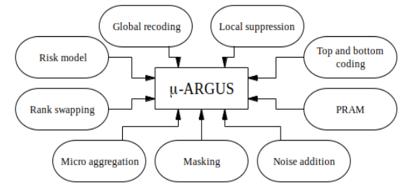
Many of the methods described previously in the methodology section can be applied with \(\mu\)-ARGUS to a dataset. It is our aim to include other methods as well in the near future, if time permits

\(\mu\)-ARGUS is a flexible interactive program that will guide you through the process of data protection. In a typically \(\mu\)-ARGUS run you will typically go through the following steps, given that the microdata set is ready.

1. Meta data. \(\mu\)-ARGUS needs to know the structure of the data set. Not only the general aspects but also additional SDC-specific information. As there is till now no suitable flexible standard for meta data allowing us to specify also the SDC-specific parts of the meta data, we have to rely on the ARGUS meta data format.
   This can be prepared (partially) externally or it can be specified interactively during a \(\mu\)-ARGUS session.
2. Threshold-rule/risk models. Selection and computation of frequency tables on which several SDC-methods (like risk models, threshold rule) are based
3. Global recoding. Selection of possible recodings and inspection of the results.
4. Selection and application of other protection methods like:
   • Microaggregation (3.4.2.3)
   • PRAM (3.4.6)
   • Rounding (3.4.2.5)
   • Top and bottom coding (3.4.3.3)
   • Rank swapping (3.4.2.4)
   • Noise addition (3.4.2.1)
5. Risk model: selection of the risk-level
6. Generate the safe micro file. During this process all data transformations specified above. This is also the moment that all remaining unsafe combinations will be protected by local suppressions. Also an extensive report will be generated.

When the above scheme has been followed a safe microdata file has been generated. \(\mu\)‑ARGUS is capable of handling very large datasets. Only during the first phase, when the datafile is explored and the frequency tables are computed some heavy computations are performed. This might take some time depending on the size of the datafile. However all the real SDC-work (global recoding and the other methods named under 4 and 5 above) are done at the level of the information prepared during this first phase. This will be done very quickly. Only in the final phase when the protected datafile is made, the operation might be time consuming depending on the size of the datafile.

This architecture of \(\mu\)‑ARGUS has the advantage that all real SDC-work, that will be done interactively, will have a very quick response time. Inspecting the results of various recodings is easy and simple.

The most recent release of \(\mu\)-ARGUS can be found on GitHub (https://github.com/sdcTools/muargus/releases).

3.6.2 sdcMicro

sdcMicro (https://github.com/sdcTools/sdcMicro) is an R package implementing almost all methods discussed in Section 3.4. The required steps to use the package are essentially the same as outlined in Section 3.6.1 and are quickly summarized below as well.

1. Definition of a problem The first step is always to create an object that defines the current sdc problem. This task can be achieved by calling function createSdcObj(). In this function, quite a few parameters can be set. The most important ones are:

   • Data: the input data set needs to be a data.frame / data.table but it should be noted that any functionality from R can be used to create such objects from a variety of files exported or generated from other tools such as SAS, SPSS or STATA among using plain text-files (such as .csv) or other structured formats like .json or .xml as long those can be converted to a rectangular data structures. It is of course also possible to use queries to database systems in order to create suitable input objects.
   • Key variables for risk assessment: the user is required to specify a set of categorical key variables. These variables are automatically used when computing risk measures (see also Section 3.3.3).
   • Numerical key variables: It is also possible (but optional) to specify a set of numerical variables that are deemed important. Such variables can (automatically) be used to apply suitable perturbation methods (such as e.g masking by noise) to it.
   • Weights: In case the underlying microdata step from a survey sample, a variable holding suitable weights can be specified. This is required in order to make sure that risk measures are computed correctly.
   • Strata: Sometimes it is useful if a specific anonymization approach is applied independently to specific strata of the underlying population. In sdcMicro this can be achieved by defining a variable that holds different values for different groups of the population.
   • Ghost-variables: This allows to link variables to (categorical key) variables in a sense that modifications to the relevant key-variable (e.g suppression) are transferred and applied to the dependent variables that are referred to as “ghost” variables
   • Excluding direct identifiers: In statistical practice microdata files often contain direct identifiers which can be identified already on creation of an input object. If such variables have been defined, they will be removed prior to any computations.

   It should be noted that while it is very convenient to work with an object created with createSdcObj(), it is perfectly possible to apply all implemented methods of the package also to simpler data-structures like a data.frame.

2. Application of SDC-methods Once a problem instance has been created, some helpful summary statistics such as the number of observations violating \(k\)-anonymity or (global) risk measures such as the expected number of re-identifications given the defined risk-scenario, are readily available and are shown by simply printing out the object.

   The next step is then to interactively apply SDC techniques to the object and re-assess the impact of its application both on risk-measures as well as on data-utility. If the application yields unexpected or bad results, the implemented undo()-method can be used to revert to the state before application of the specific methods. This allows to quickly try out different parameter settings and makes the process of applying SDC methods quite interactive.

   The package allows to (for example) add stochastic noise to numerical variables (3.4.2.1) using addNoise(), post-randomize values in categorically scaled variables (3.4.6) with function pram(), create synthetic microdata (3.4.7) with method dataGen() or perform global recoding (3.4.3.2) by using globalRecode(). Furthermore it is possible to apply rank-swapping (3.4.2.4) with function rankSwap(), compute SUDA-scores (3.3.7) using suda2(), compute individual risk estimates (3.3.5) with indivRisk() and freqCalc() as well as make a set of categorical key variables fulfill \(k\)-anonymity using kAnon(). In the current versions of the package, TRS (targeted record swapping, 5.6) is implemented and can be called using the recordSwap() function. A detailed discussion and overview is available in a custom vignette (https://sdctools.github.io/sdcMicro/articles/recordSwapping.html).

3. Exporting Results Once the interactive process has been finished, the package allows to quickly write out a safe dataset that contains all applied techniques also respecting any settings defined when initializing the object itself such as “ghost-variables” using function writeSafeFile().

   Further more there is a report() functionality available that can be applied to an sdc-object at any time. This method can be called to either generate an internal or external report summarizing the process. The difference between the internal and the external report is the level of detail. While the external report is targeted for public consumption and does not contain any (sensitive) values such as specific parameter settings, the internal report lists any techniques that have been applied to protect the microdata in great detail. Both variants result in a html file that can easily be shared.

4. Graphical User-Interface Creating safe, protected microdata files is often a challenging task. Also having to dive into R and write code to perform several steps of the procedure can be a hurdle for non-experts in R. In order to mitigate this problem and to facilitate the use of sdcMicro, the package comes with an interactive, shiny-based graphical user-interface (Meindl, 2019). The interface can be started using the sdcApp function and its functionality is explained in detail in a custom vignette (https://sdctools.github.io/sdcMicro/articles/sdcMicro.html).

3.7 Introductory example: rules at Statistics Netherlands

As has been shown in the previous sections there are many sophisticated ways of making a safe protected microdata set. And it is far from a simple straightforward task to select the most appropriate method for the Disclosure Protection of a microdata set. This requires a solid knowledge of the survey in question as well as a good overview of all the methods described in the previous sections.

However as an introduction we will describe here a method/set of rules inspired by those currently applied at Statistics Netherlands for making both microdata files for researchers as well as public use files. This approach can be easily applied, as it is readily available in \(\mu\)-ARGUS. These rules are based on the ARGUS threshold-rule in combination with global recoding and local suppression (see Section 3.4.3.2 and 3.4.3.4). This rule only concentrates on the identifying variables or key-variables, as these are the starting point for an intrusion. There rules have primarily been developed for microdata about persons.

Microdata for researchers
For the microdata for researchers one could use the following set of rules:

1. Direct identifiers should not be released and therefore should be removed from the microdata set.
2. The indirect identifiers are subdivided into extremely identifying variables, very identifying variables and identifying variables. Only direct regional variables are considered to be extremely identifying. Very identifying variable are very visible variables like gender, ethnicity etc. Each combination of values of an extremely identifying variable, a very identifying variable and an identifying variable should occur at least 100 times in the population.
3. The maximum level of detail for occupation, firm and level of education is determined by the most detailed direct regional variable. This rule does not replace rule 2, but is instead a practical extension of that rule.
4. A region that can be distinguished in the microdata should contain at least 10 000 inhabitants.
5. If the microdata concern panel data direct regional data should not be released. This rule prevents the disclosure of individual information by using the panel character of the microdata.

If these rules are violated, global recoding and local suppression are applied to achieve a safe file. Both global recoding and local suppression lead to information loss, because either less detailed information is provided or some information is not given at all. A balance between global recoding and local suppression should always be found in order to make the information loss due to the statistical disclosure control measures as low as possible. It is recommended to start by recoding some variables globally until the number of unsafe combinations that has to be protected is sufficiently low. Then the remaining unsafe combinations have to be protected by local suppressions.

For business microdata these rules are not appropriate. Opposite to personal microdata business data tends to be much more skewed. Each business is much more visible in a microdata set. This makes it very hard to make a safe business micro dataset.

Microdata for the general public
The software package \(\mu\)-ARGUS (see e.g. Hundepool et al, 2014) is also of help in producing public use microdata files. For public use microdata files one could use the following set of rules:

1. The microdata must be at least one year old before they may be released.
2. Direct identifiers should not be released. Also direct regional variables, nationality, country of birth and ethnicity should not be released.
3. Only one kind of indirect regional variables (e.g. the size class of the place of residence) may be released. The combinations of values of the indirect regional variables should be sufficiently scattered, i.e. each area that can be distinguished should contain at least 200 000 persons in the target population and, moreover, should consist of municipalities from at least six of the twelve provinces in the Netherlands. The number of inhabitants of a municipality in an area that can be distinguished should be less than 50 % of the total number of inhabitants in that area.
4. The number of identifying variables in the microdata is at most 15.
5. Sensitive variables should not be released.
6. It should be impossible to derive additional identifying information from the sampling weights.
7. At least 200 000 persons in the population should score on each value of an identifying variable.
8. At least 1 000 persons in the population should score on each value of the crossing of two identifying variables.
9. For each household from which more than one person participated in the survey we demand that the total number of households that correspond to any particular combination of values of household variables is at least five in the microdata.
10. The records of the microdata should be released in random order.

According to this set of rules the public use files are protected much more severely than the microdata for research. Note that for the microdata for research it is necessary to check certain trivariate combinations of values of identifying variables and for the public use files it is sufficient to check bivariate combinations, but the thresholds are much higher. However, for public use files it is not allowed to release direct regional variables. When no direct regional variable is released in a microdata set for research, then only some bivariate combinations of values of identifying variables should be checked according to the statistical disclosure control rules. For the corresponding public use files all the bivariate combinations of values of identifying variables should be checked.

3.8 Further examples

In this section we provide examples based on real surveys of the various steps described in the previous sections in order to describe a possible process of microdata anonymisation in practice. The two surveys analysed are one from the social domain, the Labour Force Survey (LFS), and one on business data, the Community Innovation Survey (CIS). Notice how the complexity of the reasoning on business data may rise sharply as compared to social microdata.

3.8.1 Labour Force Survey

The Labour Force Survey³ is one of the surveys subject to Regulation EC 831/2002 on access to microdata for scientific purposes. The Labour Force Survey (LFS) is the main data source for the analysis of the labour market, employment, unemployment as well as the conditions and the level of involvement at the labour market. Some of the main observed variables are:

³ The European Union Labour Force Survey (EU LFS)? is conducted in the 25 Member States of the European Union and 3 countries of the European Free Trade Association (EFTA) in accordance with Council Regulation (EEC) No. 577/98 of 9 March 98: https://eur-lex.europa.eu/legal-content/EN/ALL/?uri=celex%3A31998R0577

1. demographic variable: (gender, year of birth, marital status, relationship to reference person, place of residence);
2. labour status: (labour status during the reference week, etc.);
3. employment characteristics of the main job: (professional status, economic activity of local unit, country of place of work, etc.);
4. education and training;
5. income;
6. technical item relating to the interview.

The sampling designs in the EU-LFS are extremely varied. Most NSIs employ some kind of multistage stratified random sampling design, especially those that do not have central population register available.

In the document Eurostat (2004) a proposal for the anonymisation of the LFS is presented. Here we show a possible approach to disclosure scenario definition that leads to the definition of the identifying variables.

Disclosure scenarios
A spontaneous identification (see Section 3.3.2) can happen when an intruder has a direct knowledge of some statistical units belonging to the sample and, whether such units assume extremely particular values for some variables or for some combinations. In the Labour Force data set there are several variables that may lead to a spontaneous identification. Some of these variables are: professional status, number of persons working at local unit, income, economic activity, etc. To avoid a possible spontaneous identification such variables are usually checked to see whether there are unusual patterns or very rare keys and, if necessary some recoding or suppression may be suggested.

Also the external register scenario could be considered for the LFS data. The two external archives taken as example in the Italian study are: (i) the Electoral roll for the Individual archive scenario, and (ii) the Population register for the Household archive scenario (see Section 3.3.2). The Electoral roll is a register containing information on people having electoral rights, mainly demographic variables (gender, age, place of residence and birth) and sometimes variables such as, marital status, professional and/or educational information. The key variables considered as reliable for re‑identification attempts under this scenario are: gender, age and residence. Place of birth is removed from the MF and the others are not considered as their quality was not deemed sufficient for re-identification purposes. The Population register maybe a public register containing demographic information at individual and household level. Particularly, the set of key variables considered for the household archive scenario comprises the variables: gender, age, place of residence and marital status as individual information, the household size and parental relationship as household information.

Risk assessment
The definition of the identifying variables allows for a definition of risk assessment. This can be performed as in Eurostat (2004) following the reasoning of Section 3.7 or other risk measures can be used. If the survey employs a complex multi-staged stratified random sample design possibly with calibration, then the ARGUS individual risk may be used especially when hierarchical information on the household need to be released.

Protection
The risk assessment procedure will show the keys at risk and based on this information a strategy for microdata protection needs to be adopted. If the number of keys at risk is very large then some variables are too detailed and some global recoding is advisable in order to avoid the application of a high percentage of local suppressions. If the keys at risk are particularly concentrated on certain values of an identifying variable a local recoding of such variable could be sufficient to solve the problem.

3.8.2 Community Innovation Survey

The Community Innovation Survey is one of the surveys subject to Regulation CE 831/2002 on access to microdata for scientific purpose. A lot of effort has been put in anonymising this microdata set, see for example Eurostat (2006).

In this section we propose a study of disclosure scenarios to define identifying variables and a risk assessment analysis to single out the records at risk for the Community Innovation Survey (CIS) based on Ichim (2006). A protection stage is then outlined giving different choices. The interested reader is referred to that paper for more information on the whole process.

CIS provides information on the characteristics of innovation activity at enterprise level⁴. The CIS statistical population is determined by the size of the enterprise (all enterprises with 10 or more employees) and its principal economic activity.

⁴ Some of the main observed variables in the CIS3 are : principal economic activity, geographical information, number of employees in 1998 and 2000, turnover in 1998 and 2000, exports in 1998 and 2000, gross investment in tangible goods: 2000, number of valid patents at end of 2000, number of employees with higher education (in line with the number of employees in 2000), expenditure in intramural RD (in line with the turnover in 2000), expenditure in extramural RD (in line with the turnover in 2000), expenditure in acquisition of machinery (in line with the turnover in 2000), expenditure in other external knowledge (in line with the turnover in 2000), expenditure in training, market (in line with the turnover in 2000), total innovation expenditure (in line with the turnover in 2000), number of persons involved in intra RD (in line with the number of employees in 2000).

Disclosure scenario
Since generally business registers are publicly available, it is supposed that an intruder could use such information to identify an enterprise. Public business registers report general information on name, address, turnover (TURN), number of employees (EMP), principal activity of an enterprise (NACE), region (NUTS). Therefore, the identifying variables of the hypothesized disclosure scenario are: economic classification (NACE), region (NUTS), number of employees (EMP) and turnover (TURN). The information content of these variables must be somehow reduced in order to increase the intruder uncertainty. An initial coding performed on such variables was: NACE at 2 digits, Nuts recoded at national level (no regional breakdown) and three enterprise size classes.

Additionally, in the CIS data set there are several confidential variables that may be subject to spontaneous identification. Some examples are total expenditure on innovation (RTOT), exports, number of persons involved in intra RD, etc. Such variables are never published in an external register, but they can assume extremely particular values on some units. Mere additional information would then clearly identify an enterprise. Special attention must be paid on these variables. A check performed by the survey experts is generally suggested. These assessments must be performed with respect to each combination of categorical identifying variables to be released. The analysis by the survey expert suggested to remove from the data to be released the variable Country of head office. With the given details on NACE, size class and NUTS all the other continuous variables were not deemed sufficiently spread to lead to a spontaneous identification of a unit. For this reason it maybe suggested to let them unchanged.

Risk assessment
A unit is considered at risk if it is ‘recognisable’ either in the external register scenario or in the spontaneous identification scenario. It is assumed that an intruder may confuse a unit U with others when there is a sufficient number of units in a well-defined (and not too large) neighbourhood of U. The anonymisation proposal developed in Ichim (2006) is based on the idea that similarity based on clusters and confusion both express the same concept, although in different frameworks. : When a unit belongs to a cluster, it belongs to a high density (sufficient number of close units) subset of data. Hence the unit may be considered as being confused with others. The algorithms taking into account these two features (distance from each other and number of neighbours) are called density based algorithms and Ichim (2006) uses one of these algorithms to identify isolated units i.e. units at risk with respect to the identifying variables.

Protection by perturbation
Once the units at risk have been identified, protection should be applied. Several different proposals in the field of data perturbation methods are possible. The proposal by Eurostat protection is achieved by the application to the main continuous variables in the data set of individual ranking and some local suppression of particular values. This microaggregation would be applied to the whole file irrespective to different economic classifications or size classes and without taking into account possible relationships between variables (for example turnover needs to be greater than export or expenditures). This strategy is perfectly acceptable if a slight modification of the data is deemed sufficient.

An alternative could be to apply a perturbation only to these records at risk (mainly the large size enterprises in single NACE 2 digits) whereas the rest of the file is released unchanged. Ichim (2006) suggests different perturbations of the points at risk whereas these are in the middle of the distribution of points (nearest cluster imputation) or if they are in the tail (microaggregation). A further adjustment is proposed in order to preserve turnover totals for each combination of categorical identifying variables. This is deemed important by users who need to compare results with published tables. A study of the information loss of this approach is presented in Ichim (2006).

3.8.3 References

Eurostat (2004). Proposal on anonymised LFS microdata. CSC 2004/B5/ item 2.2.2.

Eurostat (2006). The CIS4. An amended version of the micro-data anonymisation method. Doc. Eurostat/F4/STI/CIS/M2/8.

Ichim, D. (2006). Microdata anonymisation of the Community Innovation Survey: a density based clustering approach for risk assessment. Contribution Istat. Shortly available from https://www.istat.it/wp-content/uploads/2018/07/2007_2-1.pdf

Trottini, M., Franconi, L. and Polettini, S. (2006). Italian Household Expenditure Survey: A proposal for Data Dissemination. In Domingo Ferrer, J and Franconi, L. (eds) Privacy in Statistical Databases, CENEX-SDC Project International Conference, Rome, Italy, December 2006, 318-333.