4 Magnitude tabular data
4.1 Introduction
Statistical magnitude tables display sums of observations of a quantitative variable where each sum relates to a group of observations defined by categorical variables observed for a set of respondents.
Respondents are typically companies but can also be individuals or households, etc. Grouping variables typically give information on geography or economic activity or size, etc. of the respondents. The “cells” of a table are defined by cross-combinations of the grouping variables.
Each “table cell” presents a sum of a quantitative variable such as income, turnover, expenditure, sales, number of employees, number of animals owned by farms, etc. These sums are the “cell values” (sometimes also referred to as “cell totals”) of a magnitude table. The individual observations of the variable (for each individual respondent) are the “contributions” to the cell value.
| Industry A | Industry B | … | Total | |
| Region 1 | 540 (12) | 231 (15) | … | |
| Region 2 | 48 (2) | 125 (8) | … | |
| … | … | … | … | |
| Total |
The “dimension” of a table is given by the number of grouping variables used to specify the table. We say that a table contains “margins” or “marginal cells”, if not all cells of a table are specified by the same number of grouping variables. The smaller the number of grouping variables, the higher the “level” of a marginal cell. A two-dimensional table of some business survey may for instance provide sums of observations grouped by economic activity and company size classes. At the same time it may also display the sums of observations grouped by only economic activity or by only size classes. These are then margins/marginal cells of this table. If a sum across all observations is provided, we refer to it as the “total” or “overall total”.
At first sight, one might find it difficult to understand how the kind of summary information published in magnitude tables presents a disclosure risk at all. However, it often occurs that cells of a table relate to a single or to only a few respondents. The number of this kind of small cells in a table will increase, the more grouping variables are used to specify the table, the higher the amount of detail provided by the grouping variables, and the more uneven the distributions of respondents over the categories of the grouping variables.
If a table cell relates to a small group of respondents (or even only one), then publication of the cell value may imply a disclosure risk. This is the case if these respondents could be identified by an intruder using information displayed in the table.
Example 1 Let a table cell display the turnover of companies in the mining sector for a particular region X. Let us assume that company A is the only mining company in this region. This is a fact that will be known to certain intruders (think, for instance, of another mining company B in a neighbouring region Y). So, if that table cell is published, company B would be able to disclose the turnover of company A.
In order to establish if a disclosure risk is connected to the publication of a cell value in a table, and in order to protect against this risk, data providers (like, e.g. National Statistical Institutes) should apply tabular data protection methods. In many countries this is a legal obligation to official statistical agencies. It may also be regarded as a necessary requirement in order to maintain the trust of respondents: After all, if in the instance above company A realizes that company B might, by looking into the published table, disclose the value of turnover it has reported, and if it considers this value as confidential information, it may refuse to respond to that survey in the next period, or (if the survey is compulsory) it may choose to provide incorrect or inaccurate information.
Especially for business statistics, the most popular method for tabular data protection is cell suppression . In tables protected by cell suppression, all values of cells for which a disclosure risk has been established are eliminated from the publication. Alternatively, other methods based on cell perturbation etc. may also be used to protect tabular data. While we focus in this chapter on cell suppression, we will also mention alternatives.
Section 4.2 introduces into the methodological concepts of tabular data protection. In Section 4.2.1 we present the most common methods for disclosure risk assessment for each individual cell of a table (and for special combinations of individual cells). These methods are called “primary” disclosure control methods. Table cells for which a disclosure risk has been established are called “sensitive”, “confidential”, or “unsafe” cells. Primary disclosure risk is usually assessed by applying certain sensitivity rules. Section 4.2.1 explains the concept of sensitivity rules and the most common rules.
While detailed tabulated summary information also on smaller groups of statistical objects (companies by subgroups of subsectors at the district level, households by size and income at the neighbourhood level, etc.) might be of interest to certain user groups, it is also a responsibility (maybe the most important one) of official statistics to provide summary information at a high aggregate level by producing summary statistics on large groups of a population (e.g. for all companies of an economy sector). Because of this, it is not enough to have methodologies to protect individual cells. It implies a need for the so-called “secondary” tabular data protection methodologies.
Assume that a table displays the sum of a variable “Production” by three subsectors of an economy sector. Assume that this sum is sensitive for one of the subsectors and that the table is protected by cell suppression, meaning that the confidential cell value is suppressed.
Example 1a Production (in mill. Euro)
| Sector | Subsector I | Subsector II | Subsector III |
| 56,600 | suppressed (sensitive) |
47,600 (non-sensitive) |
8,002 (non-sensitive) |
With respect to the total production for this sector we distinguish two cases: Either it is foreseen to be published – we then consider it as a cell of the table (e.g. the “total”). If the cell values of the two non-sensitive subsectors and the “total” are displayed, then users of the publication can disclose the cell value for the sensitive subsector by taking the difference between the “total” and the subsector values for the two non-sensitive sectors (56,600 – 47,600 – 8,002 = 998). In order to avoid this, a secondary protection measure for this table has to be taken, e.g. selecting one of the two non-sensitive subsector cells and suppressing it as well. This would be called a “secondary suppression”.
The other option is that the “total” is not foreseen to be displayed / published. Then no secondary protection measure would be needed. In this instance, because the production for one subsector is suppressed, interested users of the table cannot compute the production for the sector on their own – and so the sector-level information is completely lost!
From a general perspective, the purpose of secondary tabular data protection methodologies is chiefly to avoid undesirable effects such as this, ensuring that – while some “small”, primary confidential cells within detailed tables may have to be protected (by cell suppression or by some perturbative method) – sums for larger groups, i.e. the margins of those detailed tables, are preserved to some extent. For cell suppression this means that suppression of marginal cells should be avoided as far as possible. For perturbative methods it means that high level margins should try to be preserved exactly (more or less).
Considering this as the basic idea of secondary protection, after Section 4.2.1 we assume for the remainder of the chapter margins and overall totals always to be part of a table.
In Section 4.2.2 we introduce the concepts of secondary tabular data protection methodologies. The focus will be on cell suppression, but we will also mention other methodologies.
The software package \(\tau\)‑ARGUS (see e.g. Hundepool et al., 2014) provides software tools for disclosure protection methods for tabular data. The latest version of \(\tau\)-ARGUS can be found on GitHub (https://github.com/sdcTools/tauargus/releases). Section 4.3 is concerned with the practical implementation of secondary cell suppression as offered by \(\tau\)‑ARGUS. In Section 4.3.1 we discuss information loss concepts as well as table structures considered by \(\tau\)‑ARGUS. We compare the performance of different algorithms for secondary cell suppression in Section 4.3.2 and give software recommendations. In Section 4.3.3 we explain how to set up procedures for tabular data protection in a practical way and give an introductive example in Section 4.3.4. In Section 4.4 we briefly introduce the methodological concepts of the secondary cell suppression algorithms provided by \(\tau\)-ARGUS. The chapter ends with Section 4.5, introducing Controlled Tabular Adjustment as new emerging protection technique for magnitude tables which could become an alternative to the well-established cell suppression methodologies.
4.2 Disclosure Control Concepts for Magnitude Tabular Data
In this section we explain the main concepts for assessment and control of disclosure risk for magnitude tables.
Section 4.2.1 is concerned with disclosure risk for each individual cell of tables presenting summaries of quantitative variables and will introduce the most common methods used to assess this risk.
In order to preserve the margins of tables to some extent while protecting individual sensitive cells, special disclosure control methodologies have been developed. Section 4.2.2 presents basic concepts of these methodologies, focusing on secondary cell suppression as the most prominent instance. We finish section methods with a brief, comparative overview of alternative methods for tabular data protection.
4.2.1 Sensitive Cells in Magnitude Tables
We begin this section by describing intruder scenarios typically considered by statistical agencies in the context of disclosure control for magnitude tables. Considering these intruder scenarios statistical agencies have developed some ‘safety rules’ as measures to assess disclosure risks. This section will also introduce the most popular rules using some illustrative examples. Finally, we compare rules and give guidance on making a decision between alternative rules.
Intruder scenarios
If a table cell relates to a small group (or even only one) respondent, then publication of the cell value may imply a disclosure risk. This is the case, if these respondents could be identified by an intruder using information displayed in the table. In example 1 of Section 4.1, for the intruder (company B) it is enough to know that the cell value reports the turnover of mining companies in region X. In that example company B is assumed to be able to identify company A as the only mining company in region X. Hence, publication of the cell value implies a disclosure risk: if company B looks into the publication they will be able to disclose the turnover of company A.
But what if a cell value does not relate to one, but to two respondents?
Example 1b Let us assume this time that both companies (A and B) are located in region X, and are the only mining companies there. Let us further assume that they both are aware of this fact. Then again publication of the cell value implies a disclosure risk (this time to both companies): if any of the two companies look into the publication and subtract their own contribution to the cell value (i.e. the turnover they reported) from the cell value, they will be able to disclose the turnover of the other company.
Example 1c Assume now that the table cell relates to more than two respondents. Imagine this time that four companies (A, B, C and D) are located in region X. Then theoretically three of them (B, C and D, say) could form a coalition to disclose the turnover of company A. Such a coalition might be a rather theoretical construct. An equivalent but perhaps more likely scenario could be that of another party who knows the contributions of companies B, C and D (perhaps a financial advisor working for all three companies) who would then be able to disclose also the turnover of company A by subtracting the contributions of B, C and D from the cell value.
The examples above are based on the intruder scenario typical for business data: it is usually assumed, that the “intruders”, those who might be interested in disclosing individual respondent data, may be “other players in the field”, e.g. competitors of the respondent or other parties who are generally well informed on the situation in the part of the economy to which the particular cell relates. Such intruder scenarios make sense, because, unlike microdata files for researchers, tabular data released by official statistics are accessible to everybody – which means they are accessible in particular to those well informed parties.
In the scenarios of example 1 there is a risk that magnitude information is disclosed exactly. But how about approximate disclosure?
Example 1d Let us reconsider the example once more. Assume this time that in region X there are 51 companies that belong to the mining sector, e.g. company A and 50 very small companies S1 to S50. Assume further that 99 % of the turnover in mining in region X is contributed by company A. In that scenario, the cell value (turnover in the mining sector for region X) is a pretty close approximation of the turnover of company A. And even though the potential intruder (in our example mining company B of the neighbour region Y) may not be able to identify all 51 mining companies of region X, it is very likely that they will know that there is one very big company in region X and which company that is.
Sensitivity of variables
The presumption of the sensitivity of a variable often matters in the choice of a particular protection method. For example, especially in the case of tables presenting business magnitude information many agencies decide that this kind of information must be protected also against the kind of approximate disclosure illustrated by example 1d above, because it is so sensitive.
Considering the above explained intruder scenarios statistical agencies have developed some ‘safety rules’ (also referred to as ‘sensitivity rules’ or ‘sensitivity measures’), measures to assess disclosure risks. We will now introduce the most popular rules, starting with an overview presenting formal representation of these rules in Table 4.2. After that, the rules (or rather, classes of rules) will be discussed in detail. We explain in which situations it may make sense to use those rules, using simple examples for illustration where necessary.
Sensitivity rules
Table 4.2 briefly presents the most common sensitivity rules. Throughout this chapter we denote \(x_{1} \geq x_{2} \geq \cdots \geq x_{N}\) the ordered contributions by respondents \(1,2,\ldots,N\), respectively, to a cell with cell total (or cell value) \(X = \sum_{i=1}^N x_{i}\)
| Rule | Definition |
| A cell is considered unsafe, when … | |
| Minimum frequency rule | the cell frequency is less than a pre-specified minimum frequency \(n\) (the common choice is \(n=3\)). |
| \((n,k)\)-dominance rule | the sum of the \(n\) largest contributions exceeds \(k\%\) of the cell total, i.e. \[x_{1} + \ldots + x_{n} > \frac{k}{100} X \tag{4.1}\] |
| \(p\%\)-rule | the cell total minus the 2 largest contributions \(x_{1}\) and \(x_{2}\) is less than \(p\%\) of the largest contribution, i.e.1 \[X - x_{2} - x_{1} < \frac{p}{100}x_{1} \tag{4.2}\] |
1 \(X − x_{n} − \cdots − x_{2} − x_{1} < \frac{p}{100} x_{1}\) for the case of coalitions of \(n-1\) respondents, where \(n>2\)
Note that both the dominance rule and the \(p\%\)-rule are meaningful only when all contributions are non-negative. Moreover, the dominance rule does not make sense for \(k=100\) and neither does the \(p\%\)-rule for \(p = 0\). Both rules are asymptotically equal to minimum frequency rules for \(k\rightarrow 100\), or \(p \rightarrow 0\) respectively.
Both, the dominance rule and the \(p\%\)-rule belong to a class of rules which are referred to as “concentration rules” below.
When cell suppression is used to protect the table, any aggregate (or: cell in a table) that is indeed ‘unsafe’, or ‘sensitive’ according to the sensitivity rule employed, is subject to what is called ‘primary suppression’.
Choice of a particular sensitivity rule is usually based on certain intruder scenarios involving assumptions about additional knowledge available in public or to particular users of the data, and on some (intuitive) notion on the sensitivity of the variable involved.
Minimum frequency rule
When the disseminating agency thinks it is enough to prevent exact disclosure, all cells with at least as many respondents as a certain, fixed minimum frequency \(n\) are considered safe. Example 1 of Section 4.1 (cell value referring to one company in the mining sector of a region) illustrates the disclosure risk for cells with frequency 1. Example 1b above (on two mining companies) shows that there is a similar risk for cells with frequency 2.
Normally the minimum frequency \(n\) will be set to 3.
An exception is the case when for some \(n_0\) larger than 3 the agency thinks it is realistic to assume that a coalition of \(n_0 - 2\) respondents contributing to the same cell may pool their data to disclose the contribution of another respondent. In such a case we set \(n\) to \(n_0\). Example 1c above provides an instance for this case with \(n_0=5\). (The intruder knows the pooled data of \(5 - 2 = 3\) companies (e.g. B, C and D)).
It should be stressed here that a minimum frequency larger than 3 normally does not make much sense, even though in example 1c, for some cells of a table it may happen that such a ‘pooled data’ situation actually occurs. Usually there is no way for an agency to know for which cell which size to assume for the ‘pool’. Let us assume, for instance, that in a cell with 100 respondents 99 are in the stock market and are therefore obliged to publish data which are also their contributions to that cell value. Then we should consider 99 as the size of the pool, because anybody could add up (i.e. pool) these 99 published data values in order to disclose the (confidential) contribution of company 100 who is not in the stock market. But should the agency really consider all cells with less than 101 respondents as unsafe?
Concentration rules
A published cell total is of course always an upper bound for each individual contribution to that cell. This bound is the closer to an individual contribution, the larger the size of the contribution. This fact is the mathematical foundation of the well-known concentration rules. Concentration rules like the dominance and \(p\%\)‑rule make sense only if it is assumed specifically that the intruders are able to identify the largest contributors to a cell. The commonly applied sensitivity rules differ in the particular kind and precision of additional knowledge assumed to be around.
When a particular variable is deemed strongly confidential, preventing only exact disclosure may be judged inadequate. In such a case a concentration rule should be specified. For reasons that will be explained below, we recommend use of the so called \(p\%\) ‑rule. Another, well known concentration rule is the ‘\(n\) respondent, \(k\) percent’ dominance rule. Note, that it is absolutely essential to keep the parameters of a concentration rule confidential!
Traditionally, some agencies use a combination of a minimum frequency rule together with a \((1,k)\)‑dominance rule. This approach, however, is inadequate, because it ignores the problem that in some cases the contributor with the second largest contribution to a cell which is non-sensitive according to this rule is able to derive a close upper estimate for the contribution of the largest one by subtracting her own contribution from the aggregate total. Example 1 provides an instance.
Example 1 Application of the (1,90)-rule. Let the total value of a table cell be \(X = 100,000\), let the two largest contributions be \(x_{1} = 50,000\) and \(x_{2} = 49,\!000\). Since \(50,\!000 < \frac{90}{100} 100,\!000\) the cell is safe according to the \((1,90)\)-rule: there seems to be no risk of disclosure. But the second largest contributor is able to derive an upper estimate \({\hat{x}}_{1} = 100,\!000 − 49,\!000 = 51,\!000\) for the largest contribution which overestimates the true value of \(50,000\) by \(2\%\) only: quite a good estimate!
Unlike the \((1,k)\)-dominance rule, both the \((2,k)\)‑dominance rule and \(p\%\)‑rule take the additional knowledge of the second largest contributor into account properly. Of the two, the \(p\%\)‑rule should be preferred, because the \((2,k)\)-dominance rule has a certain tendency for overprotection, as we will see in the following.
\(p\%\)-rule and dominance-rule
We will show in the following that, according to both types of concentration rules, an aggregate total (i.e. cell value) \(X\) is considered as sensitive, if it provides an upper estimate for one of the individual contributions that is relatively close to this contribution.
Assume that there are no coalitions of respondents, i.e. there are no intruders knowing more than one of the contributions. Then the closest upper estimate of any other contribution can be obtained by the second largest contributor, when it subtracts its own contribution \(x_{2}\) from the aggregate total (i.e. cell value) \(X\) to estimate the largest contribution (\({\hat{x}}_{1} = X - x_{2}\)) as seen in example 1. All other scenarios of a contributor subtracting its own value from the total, to estimate another, result in larger relative error. In the, rather unlikely, scenario that \(n - 1\) (for \(n > 2\)), respondents pool their data in order to disclose the contribution of another, the closest upper estimate of any other contribution can be obtained by the coalition of respondents \(2, 3,\ldots, n\) when they estimate \({\hat{x}}_{1} = X - x_{2} - x_{3} - \ldots - x_{n}\).
The question is now, how to determine whether such an estimate is ‘relatively close’.
Application of the \(p\%\)-rule yields that the upper estimate \({\hat{x}}_{1}\) will overestimate the true value by at least \(p\%\) for any non-sensitive cell, i.e. \({\hat{x}}_{1} - x_{1} \geq \frac{p}{100} x_{1}\) . That is, the \(p\%\)‑rule sets the difference between estimate and true value of the largest contribution in relation to the value of the largest contribution itself.
When we adapt relation (4.1) in table 1 (see definition of the \((n,k)\)-rule) to the case of \(n = 2\), subtract both sides from \(X\) and then divide by \(X\) the result is \[ (X - x_{2}) - x_{1} < \frac{100 - k}{100} X \tag{4.3}\]
In this formulation, the \((2,k)\)-rule looks very similar to the formulation of the \(p\%\)-rule given by (4.2). Both rules define an aggregate to be sensitive, when the estimate \(\hat{x}_{1} = X - x_{2}\) does not overestimate the true value of \(x_{1}\) ‘sufficiently’. The difference between both rules is in how they determine this ‘sufficiency’. According to the \(p\%\)-rule, it is expressed as a rate (i.e. \(p\%\)) of the true value of the largest contribution \(x_{1}\), while according to the \((2,k)\)‑rule, it is expressed as a rate (i.e. \((100-k)\%\)) of the aggregate total \(X\). Considering this, the concept of the \(p\%\)-rule seems to be more natural than that of the \((2,k)\)-rule.
\((2,k)\)-rules correspond to \(p\%\)-rules in the following way:
If \(k\) is set to \(100 \frac{100}{100+p}\) then
any aggregate, which is safe according to the \((2,k)\)‑rule, is also safe according to the \(p\%\)-rule (this will be proven below), but
not any aggregate, which is safe according to the \(p\%\)-rule, is also safe according to this \((2,k)\)-rule. An example is given below (example 2). In these cases the aggregate could be published according to the \(p\%\)-rule, but would have to be suppressed according to the \((2,k)\)-rule.
Based on the above explained idea, that the concept of the \(p\%\)-rule is more natural than that of the \((2,k)\)-rule, we interpret this as a tendency for over-protection in the \((2,k)\)-rule. Example 2 below is an instance for this kind of over-protection.
We therefore recommend use of the \(p\%\)‑rule instead of a \((2,k)\)‑dominance rule.
How to obtain the \(p\) parameter?
When we replace a \((2,k)\)‑dominance rule, by a \(p\%\)‑rule, the natural choice is to derive the parameter \(p\) from \(k = 100 \frac{100}{100 + p}\) , e.g. to set \(p = 100 \frac{100 - k}{k}\)
Thus, a \((2,80)\)‑dominance rule would be replaced by a \(p\%\)‑rule with \(p = 25\), a \((2,95)\)‑dominance rule by a \(p\%\)‑rule with \(p = 5.26\) .
If we also derive \(p\) from this formula, when replacing a \((1,k)\)‑dominance rule, we will obtain a much larger number of sensitive cells. In addition to the cells which are unsafe according to the \((1,k)\)-dominance rule which will then also be unsafe according to the \(p\%\)‑rule, there will be cells which were safe according to the \((1,k)\)‑dominance rule, but are not safe according to the \(p\%\)‑rule, because the rule correctly considers the insider knowledge of a large second largest contributor. We could then put up with this increase in the number of sensitive cells. Alternatively, we could consider the number of sensitive cells that we used to assign (with the \((1,k)\)-dominance rule) as a kind of a maximum-price we are prepared to ‘pay’ for data protection. In that case we will reduce the parameter \(p\). The effect will be that some of the cells we used to consider as sensitive according to the \((1,k)\)-dominance rule will now not be sensitive. But this would be justified because those cells are less sensitive as the cells which are unsafe according to the \(p\%\)-rule, but are not according to the former \((1,k)\)-dominance rule, as illustrated above by Example 1.
Example 2 Let \(p = 10\), then \(k = 100 \frac{100}{100 + p} = 90.9\), let the total value of a table cell be \(X = 110,\!000\), let the largest two contributions be \(x_{1} = 52,\!000\), and \(x_{2} = 50,\!000\).
Then \[ \hat{x_1} = X - x_{2} = 110,\!000 − 50,\!000 = 60,\!000 \] and \[ 100 \frac{\hat{x_1} - x_1}{x_1}=100 \frac{60,\!000 - 52,\!000}{52,\!000}=15.4 \] i.e. the upper estimate \(\hat{x_1} = X - x_{2}\) will overestimate the true value by \(15.4\%\). So the aggregate is safe according to the \(p\%\)-rule at \(p = 10\).
On the other hand the two largest contributions are \(x_{1} + x_{2} = 102,\!000\). As \(102,000 > \frac{100} {100 + p } X = 100,\!000\) the aggregate is not safe according to the \((2,k)\)-rule.
Proof of A.
For an aggregate which is safe according to the \((2,k)\)‑rule with \(k = 100 \cdot \frac{100}{100 + p}\) the following will hold: \[
x_{1} \leq \frac{k}{100} \cdot X = \frac{100}{100 + p} X
\tag{4.4}\] and \[\frac{ \left( X - x_{2} \right) - x_{1} }{ X } \geq 1 - \frac{k}{100} = 1 - \frac{100}{100 + p} = \frac{p} {100 + p}
\tag{4.5}\] (c.f. (4.3) ).
This is equivalent to \[
\frac{ \left( X - x_{2} \right) - x_{1} }{ x_1 } \geq \frac{p}{100+p}\frac{X}{x1}
\tag{4.6}\] From (4.4) it follows that \[
\frac{ p }{ 100 + p } \frac{ X }{ x_{1} } \geq \frac{p}{100}
\] And hence from (4.6) that \[\frac{ \left( X - x_{2} \right) - x_{1} } { x_{1} } \geq \frac{p}{ 100 + p } \cdot \frac{ X }{ x_{ 1 } } \geq \frac{ p }{ 100 }
\]
The \((p,q)\)-rule
A well known extension of the \(p\%\)-rule is the so called prior‑posterior \((p,q)\)‑rule. With the extended rule, one can formally account for general knowledge about individual contributions assumed to be around prior to the publication, in particular that the second largest contributor can estimate the smaller contributions \(X_{R} = \sum_{ i > 2 } x_{i}\) to within \(q\%\). An aggregate is then considered unsafe when the second largest respondent could estimate the largest contribution \(x_{1}\) to within \(p\) percent of \(x_{1}\) , by subtracting her own contribution and this estimate \({\hat{X}}_{R}\) from the cell total, i.e. when \(|\left( X - x_{2} \right) - x_{1} - {\hat{X}}_{R}| < \frac{p}{100} x_{1}\). Because \(\left( X - x_{2} \right) - x_{1} = X_{R}\), the left hand side is assumed to be less than \(\frac{q}{100} X_{R}\). So the aggregate is considered to be sensitive, if \(X_{R} < \frac{p}{q} x_{1}\). Evidently, it is actually the ratio \(\frac{p}{q}\) which determines which cells are considered safe, or unsafe. Therefore, any \((p,q)\)‑rule with \(q < 100\) can also be expressed as \(( p^*, q^*)\)‑rule, with \(q^* = 100\) and \[
p^* := 100 \frac{p}{q}
\tag{4.7}\]
Of course we can also adapt the \((n,k)\)-dominance rule to account for \(q\%\) relative a priori bounds: Let e.g. \(n = 2\). According to (4.3) above, an aggregate should then be considered unsafe when the second largest respondent could estimate the largest contribution \(x_{1}\) to within \((100 - k)\) percent of \(X\) , by subtracting her own contribution and the estimate \({\hat{X}}_{R}\) from the cell total, i.e. when \(|\left( X - x_{2} \right) - x_{1} - {\hat{X}}_{R}| < (100 - k)/100 X\). Just as in the case of the \(p\%\)-rule, we see that the aggregate is sensitive, when \(X_{R} < \frac{100 - k}{q} X\), and that for given parameters \(k\) and \(q\) the parameter \(k^*\) corresponding to \(q^* = 100\) should be chosen such that \[ \frac{100-k^*}{100} = \frac{100-k}{q} \tag{4.8}\]
For a more analytical discussion of sensitivity rules the interested reader is referred to (Cox, 2001), for more generalized formulations considering coalitions to (Loeve, 2001).
Negative contributions
When disclosure risk has to be assessed for a variable that can take not only positive, but also negative values, we suggest to reduce the value of \(p\) (or increase \(k\), for the dominance-rule, resp.). It may even be adequate to take that reduction even to the extent of replacing a concentration rule by a minimum frequency rule. This recommendation is motivated by the following consideration. Above, we have explained that the \(p\%\)‑rule is equivalent to a \((p,q)\)-rule with \(q=100\). When contributions may take negative, as well as positive values, it makes sense to assume that the bound \(q_{-}\) for the relative deviation of a priori estimates \({\hat{X}}_{R}\) exceeds \(100\%\). This can be expressed as \(q_{-} = 100 f\), with \(f > 1\). According to (4.7) the \(p\) parameter \(p_f\) for the case of negative/positive data should be chosen as \(p_{f} = 100 \frac{p}{q_{-}} = 100 \frac{p}{100 f} = \frac{p}{f} < p\). That means particularly that for large \(f\) the \(p\%\)-rule with corresponding parameter \(p_{f}\) is asymptotically equal to the minimum frequency rule (c.f. the remark just below Table 4.2).
In case of the dominance rule, because of (4.8), \(k_{f}\) can be determined by \(\frac{100 - k_{f}}{100} = \frac{100 - k}{100 f}\), and because \(f > 1\) this means that \(k_{ f } > k\). For large \(f\) the dominance rule with parameter \(k_{ f }\) will be asymptotically equal to the minimum frequency rule.
Waivers
Sometimes, respondents authorize publication of an aggregate even if this publication might cause a risk of disclosure for their contributions. Such authorizations are also referred to as ‘waivers’. When \(s\) is the largest respondent from which no such waiver has been obtained, and \(r\) is the largest respondent except for \(s\) then for any pair \((i,j)\), \(i \neq j\) of respondents, where no waiver has been obtained from \(j\), it holds \(x_{i} + x_{j} \leq x_{r} + x_{s}\). Therefore, we will be able to deal with such a situation properly, if we reformulate the concentration rules as
\(X - x_{s} - x_{r} < \frac{p}{100} x_{s},\) for the \(p\%\)-rule,
and
\(x_{r} + x_{s} > \frac{k}{100} X,\) for the \((2,k)\)-dominance rule.
Foreign trade rules
In foreign trade statistics traditionally a special rule is applied. Only for those enterprises that have actively asked for protection of their information special sensitivity rules are applied. This implies that if the largest contributor to a cell asks for protection and contributes over a certain percentage to the cell total, that cell is considered a primarily unsafe cell.
Given the normal level of detail in the foreign trade tables the application of the standard sensitivity rules would imply that a very large proportion of the table should have been suppressed. This is considered not to be a desirable situation and for a long time there have not been serious complaints. This has led to this special rule. And this rule has a legal basis in the European regulation 638/2004 https://eur-lex.europa.eu/LexUriServ/LexUriServ.do?uri=CELEX:32004R0638:EN:HTML.
In \(\tau\)‑ARGUS special options (the request rule) have been introduced to apply this rule. The secondary cell suppression will be done in the standard way.
Holdings
In many datasets, especially economic datasets, the reporting unit is different from the entities we want to protect. Often companies have several branches in various regions. So the marginal cell may have several contributions but from one company only. Therefore it might be a mistake to think that such a cell is safe if we look only at the largest two contributors, while the largest three might belong to only one company.
We need to group the contributions from one company together to one contribution before we can apply the sensitivity rules.
There is no problem in making the cell totals because we are only interested in the sum of the contributions.
In \(\tau\)‑ARGUS it is possible to take this into account by using the holding option.
Sampling weights
Often tables are created from datasets based on sample surveys and NSIs collect a lot of their information this way. There are two reasons why disclosure risk assessment may also be necessary for a sample survey: especially in business surveys the common approach is to sample with unequal probabilities. The first is that large companies are often sampled with probability 1. Typically it will be the case for some of the aggregates foreseen for a publication that all respondents have been sampled with probability 1. In the absence of non-response, for such an aggregate, the survey data are data for the full population. Secondly even, if sampling probabilities are smaller than 1, if an aggregate relates to a strongly skewed population, and the sampling error is small, then the probability is high that the survey estimate for the aggregate total may also be a close estimate for the largest unit in that population. It makes sense therefore to assess the disclosure risk for survey sample estimates, if the sampling errors are small but the variables are strongly sensitive. The question is then, how to determine technically, if a sample survey aggregate should be considered safe, or unsafe. The following procedure is used in \(\tau\)‑ARGUS:
For sample survey data each record has a sampling weight associated with it. These sampling weights are constructed such that the tables produced from this datasets will resemble as much as possible the population, as if the table had been based on a full census.
Making a table one has to take into account these sampling weights. If the data file has a sampling weight, specified in the metadata, the table can be computed taking these weights into account. For making a cell total this is a straightforward procedure, however the sensitivity rules have to be adapted to the situation where we do not know the units of the population with the largest values.
One option is the following approximation:
Example A cell with two contributions:
100, weight 4
10, weight 7
The weighted cell value then equals (4 \(\times\) 100) + (7 \(\times\) 10) = 470. Without considering the weights there are only two contributors to the cell: one contributing 100 and another contributing 10. However by taking account of the sampling weights the individual contributions can be approximated as 100, 100, 100, 100, 10, 10, 10, 10, 10, 10 and 10. The largest two contributors are now 100 and 100. These are regarded as the largest two values for application of the safety rules. If the weights are not integers, a simple extension is applied.
Note:
This procedure cannot be applied in combination with the holding concept, because naturally for the approximate contributions it is unknown which holding they belong to.
It should also be noted here that with the above procedure it may happen that a cell is considered safe, even though the sample estimate of the cell total provides a very close estimate of the unit in the population with the largest value. Assume e.g. the sequence of values in the full population to be 900, 100, 100, and seven times 5. Then the population total would be 1135. Assume that we sampled two units, both with a value of 100, but with different probabilities so that the sampling weights for the two are 1, and 9, respectively, yielding a population estimate of 1000 which will not be sensitive according to the above procedure. If the second largest unit as an intruder subtracts her own contribution (= 100) from the population estimate she will obtain an estimate of the value of the largest unit which exactly matches the true value of 900. But there is of course a sampling error connected to this estimate and this fact should be considered by the intruder.
On the other hand, there is a certain tendency for overprotection associated to the above procedure, i.e. there is a chance that according to the above procedure an aggregate is unsafe, when in fact it is not. Assume e.g. the sequence of values in the full population to be 100, 50, 50, 1, 1. Assume we have sampled (with unequal probabilities) the unit with value 100 with a sampling weight of 2 associated to it, and one of the units with value 1 with a sampling weight of 3. According to the above procedure two values of 100 would be considered as largest contribution for an estimated cell total of 203 which according to for instance a \(p\%\)-rule would be considered as sensitive for any \(p>3\) . But in fact, even the second largest unit in the population with a value of 50 will overestimate the value 100 of the largest unit by about 50% when it subtracts her own contribution from the population estimate of 203.
This tendency for overprotection can be avoided, when, instead of the above procedure, in the case of sample surveys we replace for instance for the \(p\%\)‑rule the formulation (4.2) of Table 4.2 by the following \[ \hat{X} - x_{2}^{s} - x_{1}^{s} < \frac{p}{100} x_{1}^{s} \tag{4.9}\] where \(\hat{X}\) denote the estimated population total, and \(x_{i}^{s}\), \(i = 1,2\), the largest two observations from the sample.
The difference between this, and the above procedure is that with (4.9) we consider as intruder the respondent with the second largest contribution observed in the sample, whereas according to the above procedure, whenever the sampling weight of the largest respondent is 2 or more, an ‘artificial’ intruder is assumed who contributes as much as the largest observation from the sample.
Considering formulation (4.3) of the dominance-rule, it is straightforward to see that we can adapt (4.9) to the case of dominance‑rules by \[ x_{1}^{s} + \ldots + x_{n}^{s} > \frac{k}{100} \hat{X} \tag{4.10}\]
It is also important to note in this context that sampling weight should be kept confidential, because otherwise we must replace (4.9) by \[ \hat{X} - w_{2} x_{2}^{s} - w_{1} x_{1}^{s} < \frac{p}{100} x_{1}^{s} \tag{4.11}\]
where \(w_{i}\), \(i=1,2\), denote the sampling weights. Obviously, according to (4.11) more aggregates will be sensitive.
Considering this as the basic idea of secondary protection, after Section 4.2.1 we assume for the remainder of the chapter margins and overall totals always to be part of a table.
In Section 4.2.2 we introduce into the concepts of secondary tabular data protection methodologies.
4.2.2 Secondary tabular data protection methods
For reasons explained in the introduction of this chapter, we assume here that tables always include margins and overall totals along with their ‘inner’ cells. Thus, there is always a linear relationship between cells of a table. (Consider for instance example 1a of the introduction to this chapter: The sector result (say: \(X_T\)) is the sum of the three sub-sector results (\(X_1\) to \(X_3\)), i.e. the linear relationship between these four cells is given by the relation \(X_T = X_1 + X_2 + X_3\). As we have seen in example 1a, if it has been established that a disclosure risk is connected to the release of certain cells of a table, then it is not enough to prevent publication of these cells. Other cells must be suppressed (so called ‘complementary’ or ‘secondary’ suppressions), or be otherwise manipulated in order to prevent the value of the protected sensitive cell being recalculated through f.i. differencing.
Within this section we explain the methodological background of secondary tabular data protection methods.
At the end of the section we give a brief comparison of secondary cell suppression, partial suppression and controlled tabular adjustment as alternative disclosure limitation techniques.
When a table is protected by cell suppression, by making use of the linear relation between published and suppressed cell values in a table with suppressed entries, it is always possible for any particular suppressed cell of a table to derive upper and lower bounds for its true value. This holds for either tables with non-negative values, and those tables containing negative values as well, when it is assumed that instead of zero, some other (possibly tight) lower bound for any cell is available to data users in advance of publication. The interval given by these bounds is called the ‘feasibility interval’.
Example 3 This example (Geurts, 1992, Table 10, p 20) illustrates the computation of the feasibility interval in the case of a simple two-dimensional table where all cells may only assume non-negative values:
| 1 | 2 | Total | |
|---|---|---|---|
| 1 | \(X_{11}\) | \(X_{12}\) | 7 |
| 2 | \(X_{21}\) | \(X_{22}\) | 3 |
| 3 | 3 | 3 | 6 |
| Total | 9 | 7 | 16 |
For this table the following linear relations hold:
\[\begin{align} X_{11} + X_{12} &= 7 \quad \text{(R1)} \\ X_{21} + X_{22} &= 3 \quad \text{(R2)} \\ X_{11} + X_{21} &= 6 \quad \text{(C1)} \\ X_{12} + X_{22} &= 4 \quad \text{(C2)} \\ \end{align}\]
with \(X_{ij} \geq 0, \forall (i,j)\). Using linear programming methodology, it is possible to derive systematically for any suppressed cell in a table an upper bound \(\left(X^{\max} \right)\) and a lower bound \(\left( X^{\min} \right)\) for the set of feasible values. In the example above, for cell (1,1) these bounds are \(\left( X_{11}^{\min} \right)\) = 3 and \(X_{11}^{\max}\) = 6 .
In this simple instance, however, we do not need linear programming technology to derive this result: Because of the first column relation (C1) \(X_{11}\) must be less or equal 6, and because of the second row relation (R2) \(X_{21}\) must be less or equal 3. Therefore, and because of the first column relation (C1) \(X_{11}\) must be at least 3.
A general mathematical statement for the linear programming problem to compute upper and lower bounds for the suppressed entries of a table is given in Fischetti and Salazar (2000).
In principle, a set of suppressions (the ‘suppression pattern’) should only be considered valid, if the bounds for the feasibility interval of any sensitive cell cannot be used to deduce bounds on an individual respondent contribution contributing to that cell that are too close according to the sensitivity rule employed. For a mathematical statement of that condition, we determine safety bounds for primary suppressions. We call the deviation between those safety bounds and the true cell value ‘upper and lower protection levels’. The formulas of Table 4.4 can be used to compute upper protection levels. Out of symmetry considerations the lower protection level is often set identical to the upper protection level.
| Sensitivity rule | Upper protection level |
|---|---|
| \((1,k)\)-rule | \(\frac{100}{k}x_1 - X\) |
| \((n,k)\)-rule | \(\frac{100}{k} \cdot (x_{1} + x_{2} + \cdots + x_{n}) − X\) |
| \(p\%\)-rule | \(\frac{p}{100} \cdot x_{1} − (X − x_{1} − x_{2})\) |
| \((p,q)\)-rule | \(\frac{p}{q} \cdot x_{1} − (X − x_{1} − x_{2})\) |
Note that we recommend using protection levels of zero when instead of a concentration rule only a minimum frequency rule has been used for primary disclosure risk assessment. As explained in 4.2.1, minimum frequency rules (instead of concentration rules) should only be used, if it is enough to prevent exact disclosure only. And in such a case, a protection level of zero should be enough. Using \(\tau\)-ARGUS this can be achieved by setting the parameter ‘minimum frequency range’ to zero.
If the distance between upper bound of the feasibility interval and true value of a sensitive cell is below the upper protection level computed according to the formulas of Table 4.4, then this upper bound could be used to derive an estimate for individual contributions of the sensitive cell that is too close according to the safety rule employed, which can easily be proven along the lines of Cox (1981).
Example 4 Cell \(X = 330\) with 3 contributions of distinct respondents \(x_{1}=300,\ x_{2}=20,\ x_{3}=10\) is confidential (or ‘unsafe’) according to the \((1,85)\)- dominance rule. If the feasible upper bound \(X^{\max}\) for this confidential cell value is less than \(\frac{100}{85} \cdot x_{1} = 352.94\) , then it will provide an upper estimate for the largest contribution \(x_{1}\) which is too close according to the \((1,85)\)-dominance rule.
Example 5 proves the formula given in Table 4.4 for the case of the \(p\%\)-rule:
Example 5 Let \(X + U\) be the upper bound of the feasibility interval for a cell with cell value \(X\) . The second largest respondent can then deduce an upper bound \(x_{1}^{U}\)by subtracting its own contribution from that upper bound: \(x_{1}^{U} = X + U - x_{2}\). According to the definition of the \(p\%\)-rule proper protection means that \(x_{1}^{U} \geq \left( 1 + \frac{p}{100} \right) \cdot x_{1}\). So, if the feasibility interval provides upper protection, it must hold that \(U \geq \left( 1 + \frac{p}{100} \right) \cdot x_{1} - X + x_{2} = p/100 \cdot x_{1} - \left( X - x_{1} - x_{2} \right)\).
The distance between upper bound of the feasibility interval and true value of a sensitive cell must exceed the upper protection level; otherwise the sensitive cell is not properly protected. This safety criterion is a necessary, but not always sufficient criterion for proper protection! It is a sufficient criterion, when the largest respondent makes the same contribution also within the combination of suppressed cells within the same aggregation (a row or column relation of the table, for instance), and when no individual contribution of any respondent (or coalition of respondents) to such a combination of suppressed cells is larger than the second largest respondent’s (or coalition’s) contribution.
Cases where the criterion is not sufficient arise typically, when the only other suppressed cell within the same aggregation is a sensitive cell too (and not the marginal cell of the aggregation), or when the same respondent can contribute to more than one cell within the same aggregation. In these cases, it may turn out that the individual contribution of a respondent may still be disclosed, even though the upper bound of the feasibility interval is well away from the value of the sensitive cell to which this respondent contributes. The most prominent case is that of two cells with only one single contributor (a.k.a. ‘singletons’) within the same aggregation. No matter how large the cell values, because they both know their own contribution of course, both can use this additional knowledge to disclose the other’s contribution. For an analytical discussion of these issues see Cox(2001). In principle, a suppression pattern should not be considered as valid, when certain respondents can use their insider knowledge (on their own contribution to a cell) to disclose individual contributions of other respondents.
The problem of finding an optimum set of suppressions known as the ‘secondary cell suppression problem’ is to find a valid set of secondary suppressions with a minimum loss of information connected to it. For a mathematical statement of the secondary cell suppression problem see e.g. Fischetti and Salazar (2000).
However, cell suppression is not the only option to protect magnitude tables. As one alternative to cell suppression, ‘Partial Suppression’ has been suggested in Salazar (2003). The partial suppression problem is to find a valid suppression pattern, where the size of the feasibility intervals is minimal. The idea of the partial suppression method is to publish the feasibility intervals of the resulting suppression pattern. Because there is a perception that the majority of users of the publications prefer the statistical agencies to provide actual figures rather than intervals, and partial suppression tends to affect more cells than cell suppression, this method has not yet been implemented.
Another alternative method for magnitude table protection is known as ‘Controlled Tabular Adjustment’ (CTA) suggested for instance in Cox and Dandekar (2002), Castro (2003), or Castro and Giessing (2006). CTA methods attempt to find the closest table consistent with the constraints imposed by the set of table equations and by the protection levels for the sensitive cells, of course taking into account also bounds on cell values available to data users in advance of publication, like non-negativity. This adjusted table would then be released instead of the original table.
4.3 The \(\tau\)‑ARGUS Implementation of Cell Suppression
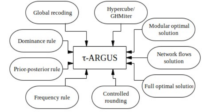
The software package \(\tau\)‑ARGUS provides software tools for disclosure protection methods for tabular data. This can be achieved by modifying the table so that it contains less, or less detailed, information. \(\tau\)‑ARGUS allows for several modifications of a table: a table can be redesigned, meaning that rows and columns can be combined; sensitive cells can be suppressed and additional cells to protect these can be found in some optimal way (secondary cell suppression). Several alternative algorithms for the selection of secondary suppressions are available in \(\tau\)‑ARGUS, e.g. the Hypercube/GHMiter method, a Modular and a Full optimal solution, and a method based on a network flow algorithm. Instead of cell suppression one could also use other methods for disclosure control of tables. One of these alternative methods is Controlled Rounding. However, use of Controlled Rounding is more common for frequency tables.
We start this section by introducing the basic issues related to the question of how to properly set up a tabular data protection problem for a given set of tables that are intended to be published, discussing tabular data structures, and particularly tables with hierarchical structures. Section 4.3.2 provides an evaluation of algorithms for secondary cell suppression offered by \(\tau\)-ARGUS, including a recommendation on which tool to use in which situation. After that, in Section 4.3.3 we give some guidance on processing table protection efficiently, especially in the case of linked tables. We finish the section with an introductive example in Section 4.3.4.
The latest version of \(\tau\)-ARGUS can be found on GitHub (https://github.com/sdcTools/tauargus/releases).
4.3.1 Setting up a Tabular Data Protection Problem in Practice
At the beginning of this section we explain the basic concept of tables in the context of tabular data protection, and complex structures like hierarchical and linked tables. In order to find a good balance between protection of individual response data and provision of information – in other words, to take control of the loss of information that obviously cannot be avoided completely because of the requirements of disclosure control, it is necessary to somehow rate the information loss connected to a cell that is suppressed. We therefore complete this section by explaining the concept of cell costs to rate information loss.
Table specification
For setting up the mathematical formulation of the protection problems connected to the release of tabulations for a certain data set, all the linear relations between the cells of those tabulations have to be considered. This leads us to a crucial question: What is a table anyway? In the absence of confidentiality concerns, a statistician creates a table in order to show certain properties of a data set, or to enhance comparison between different variables. So a single table might literally mix apples and oranges. Secondly, statisticians may wish to present a number of those ‘properties’, publishing multiple tables from a particular data set. Where does one table end and the next start? Is the ideal table one that fits nicely on a standard-size sheet of paper? With respect to tabular data protection, we have to think of tables in a different way:
Magnitude tables display sums of observations of a quantitative variable, the so-called ‘response variable’. The sums are displayed across all observations and/or within groups of observations. These groups can be formed by grouping the respondents according to certain criteria such as their economic activity, region, size class of turnover, legal form, etc. In that case the grouping of observations is defined by categorical variables observed for each individual respondent, the ’explanatory variables’. It also occurs that observations are grouped by categories of the response variable, for instance fruit production into apples, pears, cherries, etc.
The “dimension” of a table is given by the number of grouping variables used to specify the table. “Margins” or “marginal cells” of a table are those cells, which are specified by a smaller number of grouping variables. The smaller the number of grouping variables, the higher the “level” of a marginal cell. A two-dimensional table of some business survey may for instance provide sums of observations grouped by economic activity and company size classes. At the same time it may also display the sums of observations grouped by only economic activity or by only size classes. These are then margins/marginal cells of this table. If a sum across all observations is provided, we refer to it as the “total” or “overall total”.
Note that tables presenting ratios or indexes typically do not define a tabular data protection problem, because there are no additive structures between the cells of such a table, and neither between a cell value, and the values of the contributing units. Think, for instance, of mean wages, where the cell values would be a sum of wages divided by a sum over the number of employees of several companies. However, there may be exceptions: if, for instance, it is realistic to assume that the denominators (say, the number of employees) can be estimated quite closely, both on the company level and on the cell level, then it might indeed be adequate to apply disclosure control methods based, for example, on the enumerator variable (in our instance: the wages).
Hierachical, linked tables
Data collected within government statistical systems must meet the requirements of many users, who differ widely in the particular interest they take in the data. Some may need community-level data, while others need detailed data on a particular branch of the economy but no regional detail. As statisticians, we try to cope with this range of interest in our data by providing the data at several levels of detail. We usually combine explanatory variables in multiple ways, when creating tables for publication. If two tables presenting data on the same response variable share some categories of at least one explanatory variable, there will be cells which are presented in both tables – those tables are said to be linked by the cells they have in common. In order to offer a range of statistical detail, we use elaborate classification schemes to categorize respondents. Thus, a respondent will often belong to various categories of the same classification scheme ‑ for instance a particular community within a particular county within a particular state ‑ and may thus fall into three categories of the regional classification.
The structure between the categories of hierarchical variables also implies sub-structure for the table. When, in the following, we talk about sub-tables without substructure, we mean a table constructed in the following way:
For any explanatory variable we pick one particular non-bottom-level category (the ‘food production sector’ for instance). Then we construct a ‘sub-variable’. This sub-variable consists only of the category picked in the first step and those categories of the level immediately below belonging to this category (bakers, butchers, etc.). After doing that for each explanatory variable the table specified through a set of these sub-variables is free from substructure then, and is a sub-table of the original one. Any cell within the sub-table does also belong to the original table. Many cells of the original table will appear in more than one sub-table: The sub-tables are linked. Example 6 provides a simple instance of a one-dimensional table with hierarchical structure.
Example 6 Assume the categories A, AA, AB, AB1, AB2, and AB3 of some variable EXP resemble a hierarchical structure as depicted in Figure 4.2 below:
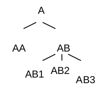
Let the full table present turnover by the categories of EXP. Then the two subtables of this table will be:
| EXP | Turnover | |
| A | ||
| AA | ||
| AB |
| EXP | Turnover | |
| AB | ||
| AB1 | ||
| AB2 |
Note that cell AB appears in both subtables
Of course, when using cell suppression methods to protect a set of linked tables, or sub-tables, it is not enough to select secondary suppressions for each table (or sub-table) separately. Otherwise it might for instance happen that the same cell is suppressed in one table because it is used as secondary suppression, while within another table it remains unsuppressed. A user comparing the two tables would then be able to disclose confidential cells in the first table. A common approach is to protect tables separately, but note any complementary suppression belonging also to one of the other tables; suppress it in this table as well, and repeat the cell suppression procedure for this table. This approach is called a ‘backtracking procedure’. Although within a backtracking process for a hierarchical table the cell-suppression procedure will usually be repeated several times for each sub-table, the number of computations required for the process will be much smaller than when the entire table is protected all at once.
It must however be stressed, that a backtracking procedure is not global according to the denotation in Cox (2001). See Cox (2001) for discussion of problems related to non-global methods for secondary cell suppression.
For mathematical formulation of linked tables structures see de Wolf (2007) and de Wolf, Giessing (2008).
Cell costs
The challenge of tabular data protection is to preserve as much information in the table as possible, while creating the required uncertainty about the true values of the sensitive cells, as explained in the previous section. It is necessary to somehow rate the information content of data, in order to be able to express the task of selecting an ‘optimal set’ of secondary suppressions, or, alternatively, of adjusting a table in an optimal way, as mathematical programming problem. Information loss is expressed in these mathematical models as the sum of costs associated to the secondary suppressions, or non-sensitive cells subject to adjustment.
For cell suppression, the idea of equating a minimum loss of information with the smallest number of suppressions is probably the most natural concept. This would be implemented technically by assigning identical costs to each cell. Yet experience has shown that this concept often yields a suppression pattern in which many large cells are suppressed, which is undesirable. In practice other cost functions, based on cell values, or power transformations thereof, or cell frequencies yield better results. Note that several criteria, other than the numeric value, may also have an impact on a user’s perception of a particular cells importance, such as its situation within the table (totals and sub-totals are often rated as highly important), or its category (certain categories of variables are often considered to be of secondary importance). \(\tau\)-ARGUS offers special facilities to choose a cost function and to carry out power transformations of the cost function:
Cost function
The cost function indicates the relative importance of a cell. In principle the user could attach a separate cost to each individual cell, but that will become a rather cumbersome operation. Therefore in \(\tau\)‑ARGUS a few standard cost functions are available2:
2 One of the secondary cell suppression methods of \(\tau\)-ARGUS, the hypercube method, uses an elaborate internal weighting scheme in order to avoid to some extent the suppression of totals and subtotals which is essential for the performance of the method. In order to avoid that this internal weighting scheme is thrown out of balance, it has been decided to make the cost function facilities of t-ARGUS inoperational for this method.
- Unity, i.e. all cells have equal weight (just minimising the number of suppressions)
- The number of contributors (minimising the number of contributors to be hidden)
- The cell value itself (preserving as much as possible the largest – usually most important – cells)
- The cell value of another variable in the dataset (this will be the indication of the important cells).
Especially in the latter two cases the cell value could give too much preference to the larger cells. Is a 10 times bigger cell really 10 times as important? Sometimes there is a need to be a bit more moderate. Some transformation of the cost function is desired. Popular transformations are square-root or a log-transformation. Box and Cox (1960) have proposed a system of power transformations:
\[ y = \frac{x^{\lambda} -1}{\lambda} \]
In this formula \(\lambda = 0\) yields to a log-transformation and the \(-1\) is needed for making this formula continuous in \(\lambda\).
This last aspect and the fact that this could lead to negative values we have introduced a simplified version of the lamda-transformation in \(\tau\)‑ARGUS
\[ y = \begin{cases} x^{\lambda} \quad &\text{for }\lambda\neq0 \\ \text{log}(x)\quad &\text{for }\lambda=0 \end{cases} \]
So choosing \(\lambda = \frac{1}{2}\) will give the square-root.
4.3.2 Evaluation of Secondary Cell Suppression algorithms offered by \(\tau\)‑ARGUS
The software package \(\tau\)−ARGUS offers a variety of algorithms to assign secondary suppressions which will be described in detail in Section 4.4. While some of those algorithms are not yet fully developed, or not yet fully integrated into the package, respectively, two are indeed powerful tools for automated tabular data protection. In this section we focus on those latter algorithms. We compare them with respect to quality aspects of the protected tables, while considering also some practical issues. Based on this comparison, we finally give some recommendation on the use of those algorithms.
We begin this section by introduction of certain minimum protection standards PS1, and PS2. We explain why it is a ‘must’ for an algorithm to satisfy those standards in order to be useable in practice. For those algorithms that qualify ‘useable’ according to these criteria, we report some results of studies comparing algorithm performance with regard to information loss, and disclosure risk.
In Section 4.2.2 we have defined criteria for a safe suppression pattern. It is of course possible to design algorithms that will ensure that no suppression pattern is considered feasible unless all of these criteria are satisfied. In practice, however, such an algorithm would either require too much computer resource (in particular: CPU time) when applied to the large, detailed tabulations of official statistics, or the user would have to put up with a strong tendency for oversuppression. In the following, we therefore define minimum standards for a suppression pattern that is safe w.r.t. the safety rule adopted except for a residual disclosure risk that might be acceptable to an agency. It should be noted that those standards are definitely superior, or at least equal to what could be achieved by the traditional manual procedures for cell suppression, even if carried out with utmost care! For the evaluation, we consider only those algorithms that ensure validity of the suppression pattern at least with respect to those relaxed standards.
Minimum protection standards
For a table with hierarchical substructure, feasibility intervals computed on basis of the set of equations for the full table normally tend to be much closer than those computed on basis of separate sets of equations corresponding to sub-tables without any substructure. Moreover, making use of the additional knowledge of a respondent, who is the single respondent to a cell (a so called ‘singleton’), it is possible to derive intervals that are much closer than without this knowledge3.
3 Consider for instance the table of example 3 in Section 4.2.2. Without additional knowledge the bounds for cell (1,1) are \(X_{11}^\text{min} = 3\) and \(X_{11}\text{max} = 6\). However, if cell (1,2) were a singleton-cell (a cell with only a single contributor) then this single contributor could of course exactly compute the cell value of cell (1,1) by subtracting her own contribution from the row total of row 1.
Based on the assumption of a simple but probably more realistic disclosure scenario where intruders will deduce feasibility intervals separately for each sub-table, rather than taking the effort to consider the full table, and that single respondents, using their special additional knowledge, are more likely attempting to reveal other suppressed cell values when they are within the same row or column (more general: relation), the following minimum protection standards (PS) make sense:
(PS1) Protection against exact external disclosure:
With a valid suppression pattern, it is not possible to disclose the value of a sensitive cell exactly, if no additional knowledge (like that of a singleton) is considered, and if subsets of table equations are considered separately, i.e. when feasibility intervals are computed separately for each sub-table.(PS2) Protection against singleton disclosure:
A suppression pattern, with only two suppressed cells within a row (or column) of a table is not valid, if each of the two corresponds to a single respondent who are not identical.(PS1*) extension of (PS1) for inferential (instead of exact) disclosure,
(PS2*) extension of (PS2), covering the more general case where a single respondent can disclose another single respondent cell, not necessarily located within the same row (or column) of the table.
\(\tau\)-ARGUS offers basically two algorithms, Modular and Hypercube, both satisfying the above-mentioned minimum standards regarding disclosure risk. Both take a backtracking approach to protect hierarchical tables within an iterative procedure: they subdivide hierarchical tables into sets of linked, unstructured tables. The cell suppression problem is solved for each subtable separately. Secondary suppressions are coordinated for overlapping subtables.
The Modular approach, a.k.a. HiTaS algorithm (see de Wolf, 2002), is based on the optimal solution as implemented by Fischetti and Salazar-González. By breaking down the hierarchical table in smaller non-structured subtables, protecting these subtables and linking the subtables together by a backtracking procedure the whole table is protected. For a description of the modular approach see Section 4.4.2, the optimal Fischetti/Salazar-González method is described in section Section 4.4.1. See also Fischetti and Salazar-González (2000).
The Hypercube is based on a hypercube heuristic implemented by Repsilber (2002). See also the descriptions of this method in Section 4.4.4.
Note that in the current implementation of \(\tau\)-ARGUS, use of the optimization tools requires a license for additional commercial software (LP-solver), whereas use of the hypercube method is free. While Modular is only available for the Windows platform, of Hypercube there are also versions for Unix, IBM (OS 390) and SNI (BS2000).
Both Modular and Hypercube provide sufficient protection according to standards PS1* (protection against inferential disclosure) and PS2 above. Regarding singleton disclosure, Hypercube even satisfies the extended standard PS2*. However, simplifications of the heuristic approach of Hypercube cause a certain tendency for oversuppression. This evaluation therefore includes a relaxed variant that, instead of PS1*, satisfies only the reduced standard PS1, i.e. zero protection against inferential disclosure. We therefore refer to this method as Hyper0 in the following. Hyper0 processing can be achieved simply by deactivating the option “Protection against inferential disclosure required” when running Hypercube out of \(\tau\)‑ARGUS.
| Algorithm | Modular | Hypercube | Hyper0 | |
| Procedure for secondary suppression | Fischetti/Salazar optimization | Hypercube heuristic | ||
| Protection standard | Interval/Exact disclosure | PS1* | PS1* | PS1 |
| Singleton | PS2 | PS2* | PS2* | |
In the following, we briefly report results of two evaluations studies, in the following referred to as study A, and study B. For further detail on these studies see Giessing (2004) for study A, and Giessing et al. (2006) for study B. Both studies are based on tabulations of a strongly skewed magnitude variable.
For study A, we used a variety of hierarchical tables generated from the synthetic micro‑data set supplied as CASC deliverable 3-D3. In particular, we generated 2- and 3-dimensional tables, where one of the dimensions had a hierarchical structure. Manipulation of the depth of this hierarchy resulted in 7 different tables, with a total number of cells varying between 460 and 150,000 cells. Note that the Hyper0 method was not included in study A.
For study B, which was carried out on behalf of the German federal and state statistical offices, we used 2-dimensional tables of the German turnover tax statistics. Results have been derived for tables with 7-level hierarchical structure (given by the NACE economy classification) of the first dimension, and 4‑level structure of the second dimension given by the variable Region.
We compare the loss of information due to secondary suppression in terms of the number and cell values of secondary suppression, and analyze the disclosure risk of the protected tables. Table 4.6 reports the results regarding the loss of information obtained in study A.
| Table Hier. levels | No. Cells | No. Suppressions (%) | Added Value of Suppressions (%) | |||
|---|---|---|---|---|---|---|
| Hypercube | Modular | Hypercube | Modular | |||
| 2-dimensional tables | ||||||
| 1 | 3 | 460 | 6.96 | 4.35 | 0.18 | 0.05 |
| 2 | 4 | 1,050 | 10.95 | 8.29 | 0.98 | 0.62 |
| 3 | 6 | 8,230 | 14.92 | 11.48 | 6.78 | 1.51 |
| 4 | 7 | 16,530 | 14.97 | 11.13 | 8.24 | 2.12 |
| 3-dimensional tables | ||||||
| 5 | 3 | 8,280 | 14.63 | 10.72 | 6.92 | 1.41 |
| 6 | 4 | 18,900 | 17.31 | 15.41 | 12.57 | 3.55 |
| 7 | 6 | 148,140 | 15.99 | 10.63 | 23.16 | 3.91 |
Table 4.7 presents information loss results from study B on the two topmost levels of the second dimension variable Region, e.g. on the national, and state level.
| Algorithm for secondary suppression | Number | Added Value | |||
|---|---|---|---|---|---|
| State level | National level | overall | |||
| abs | % | abs | % | % | |
| Modular | 1,675 | 10.0 | 7 | 0.6 | 2.73 |
| Hyper0 | 2,369 | 14.1 | 8 | 0.7 | 2.40 |
| Hypercube | 2,930 | 17.4 | 22 | 1.9 | 5.69 |
Both studies show that best results are achieved by the modular method, while using either variant of the hypercube method leads to an often quite considerable increase in the amount of secondary suppression compared to the result of the modular method. The size of this increase varies between hierarchical levels of the aggregation: on the higher levels of a table the increase tends to be even larger than on the lower levels. Considering the results of study B presented in Table 4.7, on the national level we observe an increase of about 214% for Hypercube (14% for Hyper0), compared to an increase of 75% (41%) on the state level. In Giessing et al. (2006) we report also results on the district level. On that level the increase was about 28% on the higher NACE levels for Hypercube (9% for Hyper0), and 20 % for Hypercube (14% for Hyper0) on the lower levels. In study A we observed increases mostly around 30% for Hypercube, for the smallest 2‑dimensional, and the largest 3-dimensional instance even of 50% and 60%, respectively. In particular, our impression is that the hypercube method tends to behave especially badly (compared to Modular), when tabulations involve many short equations, with only a few positions.
A first conclusion from the results of study B reported above was, because of the massive oversuppression, to exclude the Hypercube method in the variant that prevents inferential disclosure from any further experimentation. Although clearly only second-best performer, testing with Hyper0 was to be continued, because of technical and cost advantages mentioned above.
In experiments with state tables where the variable Region was taken down to the community level, we found that this additional detail in the table caused an increase in suppression at the district level of about 70 – 80% with Hyper0 and about 10 – 30% with Modular.
Disclosure risk
As explained in Section 4.2.2, in principle, there is a risk of inferential disclosure, when the bounds of the feasibility interval of a sensitive cell could be used to deduce bounds on an individual respondent’s contribution that are too close according to the method employed for primary disclosure risk assessment. However, for large, complex structured tables, this risk is rather a risk potential, not comparable to the disclosure risk that would result from a publication of that cell. After all, the effort connected to the computation of feasibility intervals based on the full set of table equations is quite considerable. Moreover, in a part of the disclosure risk cases only insiders (other respondents) would actually be able to disclose the individual contribution.
Anyway, with this definition, and considering the full set of table equations, in study B we found between about 4% (protection by Modular) and about 6% (protection by Hyper0) of sensitive cells at risk in an audit step where we computed the feasibility intervals for a tabulation by NACE and state, and for two more detailed tables (down to the district level) audited separately for two of the states. In study A, we found up to about 5.5% (1.3%) cells at risk for the 2-dimensional tables protected by Modular (Hypercube, resp.), and for the 3-dimensional tables up to 2.6% (Modular) and 5.6% (Hypercube).
Of course, the risk potential is much higher for at-risk cells when the audit is carried out separately for each subtable without substructure, because the effort for this kind of analysis is much lower. Because Modular protects according to PS1* standard, there are no such cells in tables protected by Modular. For Hyper0, in study B we found about 0.4% cells at risk, when computing feasibility intervals for several subtables of a detailed tabulation.
For those subtables, when protected by Modular, for about 0.08% of the singletons, it turned out that another singleton would be able to disclose its contribution. Hyper0 satisfies PS2* standard, therefore of course no such case was found, when the table was protected by Hyper0.
Recommendation
The methods Modular and Hypercube of \(\tau\)‑ARGUS are powerful tools for secondary cell suppression. Concerning protection against external disclosure both satisfy the same protection standard. However, Modular gives much better results regarding information loss. Even compared to a variant of Hypercube (Hyper0) with relaxed protection standard, Modular performs clearly better. Although longer computation times for this method (compared to the fast hypercube method) can be a nuisance in practice, the results clearly justify this additional effort – after all, it is possible, for instance, to protect a table with detailed hierarchical structure in two dimensions and more than 800,000 cells within just about an hour. Considering the total costs involved in processing a survey, it would neither be justified to use Hypercube (or Hyper0) only in order to avoid the costs for the commercial license which is necessary to run the optimization tools of Modular.
We also recommend use of Modular to assign secondary suppressions in 3-dimensional tables. However, when those tables are given by huge classifications, long computation times may become an actual obstacle. It took us, for instance, about 11 hours to run a 823 x 18 x 10 table (first dimension hierarchical). The same table was protected by Hyper0 within about 2 minutes. Unfortunately, replacing Modular by Hyper0 in that instance leads to about 28% increase in the number of secondary suppressions.
According to our findings, we would expect the Hypercube method (i.e. Hyper0) to be good alternative to Modular, if
- Tabulations involve more than 2 dimensions and are very large, and
- the majority of table equations (e.g. rows, columns, …) are long, involving many positions, and
- the distribution of the variable which is tabulated is rather even, not skewed, resulting in a lower rate of sensitive cells, and
- protection against inferential disclosure is not an important issue, for instance when a minimum frequency rule instead of a concentration rule is employed to assess the primary disclosure risk.
In the next section we will give some hints on what to do, if according to these conditions use of the Modular method seems to not be an option, because table sizes are too large, in order to avoid being confined to the use of Hyper or Hyper0.
Concerning protection against singleton (insider) disclosure, the Hypercube method fulfils a higher standard. However, our empirical results confirm that in practice there are very few singleton cells left unprotected by Modular against this kind of disclosure risk. We are therefore confident that the problem can be fixed easily by a specialized audit step that would not even involve linear programming methods.
4.3.3 Processing table protection efficiently
Within this section we give some guidance for how to facilitate disclosure analysis, and how to use the methods of \(\tau\)-ARGUS in an efficient way. For more tips and tricks to improve practical performance, see van der Meijden (2006).
Especially in large tables with detailed hierarchical structure we have observed that the choice of the parameter lambda (\(\lambda\)) may substantially affect the suppression pattern – and the results may be unexpected. Normally we would expect that constant cell costs will lead to a solution with a (relatively) small number of secondary suppressions. In hierarchical tables, however, it may turn out that given this cost function the Modular method tends to suppress cells in the margins of subtables rather than inner cells which in turn require additional suppressions in a (linked) subtable. This effect may be so strong that in the end, a \(\lambda\) close to zero yielding approximately constant costs may lead to a larger number of suppressions as if a larger \(\lambda\) (say: 0.5) had been chosen. For larger tables it makes therefore sense to test the outcome with different values of \(\lambda\).
Table design
In Section 4.3.1 we already discussed how to set up tables for tabular data protection. If the concept for the publication is not yet fixed, some table-redesign may help to reduce the complexity of the problem.
Table redesign
If a large number of sensitive cells are present in a table, it might be an indication that the spanning variables are too detailed. In that case one could consider combining certain rows and columns in the table. (This might not always be possible because of publication policy.) Otherwise the number of secondary cell suppressions might just be too enormous. It is a property of the sensitivity rules that a joint cell is safer than any of the individual cells. So as a result of this operation the number of unsafe cells is reduced. One can try to eliminate all unsafe combinations in this way, but that might lead to an unacceptably high information loss. Instead, one could stop at some point, and eliminate the remaining unsafe combinations by using other techniques such as cell suppression.
In practice, it may also often be considered impractical and also not adequate to do the disclosure analysis for each table of the entire publication separately. A well-known simplification is to focus the analysis on certain lead variables. These lead tables are protected with \(\tau\)‑ARGUS as described above and the pattern found is then used for all the other tables. This strategy has the advantage that it is efficient and prevents the recalculation of suppressed cells by using the inherent relations between the different tables in the publication. The fact that for certain cells in the other tables not always all cells that should be considered unsafe according to the concentration rules will actually be considered unsafe, is considered a minor problem.
A compromise between the copying of the suppression pattern and protecting each table individually is the coordination of the primary suppressions only. This strategy is supported by the concept of shadow variables in \(\tau\)‑ARGUS. The shadow variable is used for the lead-table and only for finding the primary unsafe cells. After that the pattern is used for each individual table itself and the secondary cell suppression is done in the traditional way.
Shadow variables
The whole theory of primary unsafe cells is based on the idea that certain larger contributors in a cell might be at risk and need protection. The largest contributors therefore play an important role in the sensitivity rules.
Often the cell value itself is a very good estimate of the size of the contributors. But sometimes the cell value of a table is not always the best indicator of the size of the company. E.g. if the cell value is the investment in some commodity, the largest companies do not always have the largest values. Simply applying the sensitivity rules could yield a situation in which a rather small company will dominate the cell and force it to become unsafe. If we assume that this smaller company is not very well known and visible there is no reason to protect this cell.
If we want to protect the real large companies it could be a good idea to apply the sensitivity rules on another table (shadow variable) with the same spanning variables (e.g. turnover) and use the pattern of primary unsafe cells. Copy the pattern to the current table and compute the secondary unsafe cells in the normal way.
In \(\tau\)‑ARGUS we call the table where the primary unsafe cells are computed the shadow table.
Another reason for using a shadow variable could be the coordination of the pattern in different tables with the same spanning variables based on one dataset. See the remarks on periodical datasets below.
Ignore response variable relations
A commonly used strategy to simplify disclosure analysis is not to reflect the full linear relationship between published tabulation cells in the table protection procedure. A typical case, where this would be justified is the following: Assume we publish salaries of seasonal workers from foreign countries (\(S_{\text{foreigners}}\)), and also salaries of all seasonal workers (\(S_{\text{S-W}}\)), by region, for instance. Normally, for table protection we should consider the relation
\[ S_{\text{S-W}} = S_{\text{foreigners}} + S_{\text{non-foreigners}} \ , \qquad \text{(R1)} \]
even if we are not interested in publishing \(S_{\text{non-foreigners}}\) data, and may not even have collected them. Typically \(S_{\text{S-W}}\) data would also appear in other relations, for instance together with data for permanent workers as
\[ S_{\text{all}}= S_{\text{S-W}} + S_{\text{permanent}} \ , \qquad \text{(R2)} \]
so we would have to protect a set of linked tables. From a practical point of view this is of course not desirable. We assume now that \(S_{\text{non-foreigners}}\) figures are for all regions much larger as \(S_{\text{non-foreigners}}\) figures and that the \(S_{\text{non-foreigners}}\) are not published. Then the \(S_{\text{S-W}}\) figures cannot be used to estimate a sensitive \(S_{\text{foreigners}}\) cell value. It is thus not necessary to coordinate the suppression pattern for \(S_{\text{S-W}}\) and \(S_{\text{foreigners}}\). This means that it is not necessary to carry out tabular data protection for the (R1) by Region tabulation. It is enough to protect two separate tables: \(S_{\text{S-W}}\) or (R2) by Region, and \(S_{\text{foreigners}}\) by Region.
This has been an instance of how to avoid a linked-tables structure. Those structures can, on the other hand, be very useful to make tabular data protection problems tractable in practice.
Splitting detailed tables
Assume we have collected data on labour costs, including information on NACE category, Region, and Size class of the number of employees. We may want to release a 3-dimensional tabulation of labour costs by NACE, Region and Size Class. Looking at this table however, we may realize that while for a certain section (say: NACE\(_1\)) of the economy this amount of detail may be adequate, for the others (NACE\(_2\), NACE\(_3\), \(\ldots\), NACE\(_n\)) it is not: In those sections many of the lower-level cells are either empty, or sensitive. As pointed out at the end of the section on information loss of Section 4.3.2, more detail in a tabulation generally leads to more suppressions on the higher levels. This kind of oversuppression can be avoided by taking a splitting approach, splitting the table into a set of linked tables: Instead of one table, we protect three: 1.) Labour costs by Region, Size Class and NACE\(_1\), 2.) Labour costs by Region and NACE, and 3.) Labour costs by size class and NACE. Even though we cannot then release any labour cost data for a particular NACE category, in a particular Region and in a particular Size Class unless the NACE category belongs to NACE\(_1\), the additional unsuppressed information gained by means of the splitting approach (as compared to the simple approach dealing with a single 3-dimensional table only) is usually rated much higher.
Use of hierarchical structures
Especially when working with the Modular method for secondary cell suppression, using hierarchically structured variables usually helps a lot to reduce computational complexity, and hence computing time. Smaller numbers of categories per equation will make the program run faster. For the hypercube method, this is less of an issue. Here it is generally good to avoid structures with very few categories within a relation. The method has been developed for large tables, where the number of categories per relation is usually less than 20.
How to process linked tables
We explain now a way how to process a set of linked tables, for instance \(T_1\), \(T_2\), \(T_3\) using Modular for secondary cell suppression. This process is normally an iterative process. The method described here is referred to as “traditional method” in de Wolf, Giessing (2008). De Wolf, Giessing (2008) suggest an extension of the \(\tau\)‑ARGUS Modular (referred to as “adapted Modular”) method as a much more practical approach to deal with linked tables. Once this extension is available the method described in the following should be used only in cases where the adapted Modular method cannot be applied to the full set of linked tables (e.g. if the tables involve too many dimensions).
The question is then, which protection levels (cf. Section 4.2.2) to assign to those ‘manually unsafe cells’ (in the \(\tau\)‑ARGUS terminology). A proper method would consist of using a CTA method (c.f. Section 4.2.2) to find the closest adjusted table \(T_1^*\) to \(T_1\) that is consistent with the suppression pattern \(S_{11}\) (that is, all cell values of \(T_1^*\) cells that are not in \(S_{11}\) must be identical to the original \(T_1\) cell values), and the constraints imposed by the protection levels for the sensitive cells. We could then compute protection levels for \(S_{11}\) cells on basis of the distances between adjusted and original cell value. In practice a much simpler approach is usually taken, by assigning a fixed percentage (the ‘manual safety range’ \(\tau\)-ARGUS terminology) of the cell value as protection level. There is, however, no way to tell which percentage would be suitable: when a small cell is a secondary suppression for a large, strongly sensitive cell, a protection level even of 100% may be required. On the other hand, when a large cell is a secondary suppression for a very small sensitive cell, even 1% may cause overprotection.
After processing \(T_2\) in this fashion, \(T_3\) is processed. In addition to the \(S_{113}\) cells, here we also have to consider as additional suppressions \(S_{213}\) cells, i.e. the subset of secondary suppressions selected for Table \(T_2\) during the first iteration which are identical to a cell in \(T_3\).
In this way, when processing table \(T_i,\ (i = 1,2,3)\) in iteration step \(k_0\), we consider as additional suppressions \(\bigcup\limits_{k < k_{0}}{\left( S_{1\text{ki}} \cup S_{2\text{ki}} \cup S_{3\text{ki}} \right)} \cup \bigcup\limits_{j < i}{S_{\text{jk}_{0}i}}\), while we may try to avoid (by weighting, or by setting cell status to ‘protected’) that those cells that the tables have in common, i.e. the cells of \(T_{i_{j}} \quad (j \neq i)\), and that are not already contained in the set of additional suppressions are selected as secondary suppressions. Note that we assign 0% protection levels to cells in \(S_{iki}\), the set of secondary suppression which have been assigned to the current table in a previous step \(k\) of the iteration. The process is continued until for each of the tables the set of additional suppressions that has to be considered when processing the table in this step is identical to the set considered in the previous step.
The necessary modifications of cell properties like cell status, or cell costs can be achieved relatively easily using the a priori file facility of \(\tau\)-ARGUS. The general concept of this file is outlined in the following.
A-priori file
Through the standard sensitivity rules and other options we can apply all kinds of SDC-methods. Nevertheless there are situations which still require ‘manual’ intervention. E.g. for some other outside reason a cell must be suppressed or contrarily must be excluded from secondary suppression. Examples are the exports of certain sensitive goods (military equipment) to certain countries. These cells must be suppressed. Sometimes a cell value is known already to outsiders (maybe by other publications etc.) and therefore cannot be selected as a secondary suppression.
Also the preferences for the selection of the secondary suppressions via the cost function could be used as an option to influence the secondary suppression pattern. This might be the result of the year-to-year periodical data issue (see below).
Specifying all this information manually during a \(\tau\)‑ARGUS run for a large table can be rather cumbersome and error-prone. In the batch version of \(\tau\)‑ARGUS it is even impossible to do this. So the a-priori file has been introduced.
In this file the user can specify for each cell (by giving the values of the spanning variables):
cells that cannot be selected as secondary suppressions
cells that must be suppressed
specify a new value of the cost function for a cell; this can be either high or low. This will influence the chance of a cell as a candidate for sec. suppression.
Note that this option is not valid for the hypercube, as the hypercube has its own cost function that cannot be influenced.
Further details of this file can be found in the \(\tau\)‑ARGUS manual.
Periodical data
If tables are provided regularly (say monthly, quarterly or annually) certain problems may be connected to disclosure control: Firstly, it may seem to be too much effort. Secondly, if we do disclosure analysis independently each time, suppression patterns may differ. We will have the situation that we publish a particular cell value for one period, but use it as secondary suppression in the next period. Also with a cell published in one period, but becoming a primary cell in the second period, there is a risk of a very narrow estimate based on the previous period. Especially if the observations tend to be rather constant over time the pre-period value might be a close estimate of the suppressed value for the current period, which then might be used to disclose a current-period sensitive cell.
An alternative might be simply to copy the suppression pattern of the previous period, and add some (primary and secondary – if required) suppressions for those cases where cells were not sensitive in the last period, but are sensitive in the current period. Another option would be to assign low costs to previous-period suppressions when assigning secondary suppressions to the current data tables. However, both these strategies will cause an increase in information loss, which will be stronger the more changes there are in cell sensitivity between periods.
Tables with negative values
In Section 4.2.1 we already discussed the problem of negative contributions, presenting an idea on how to solve the problem with respect to primary protection. However, when there are negative contributions, it may also happen that some of the table cell values turn out to be negative. The current version of \(\tau\)-ARGUS does not yet support the processing of such a table, but a little pre-processing may solve the problem:
If the microdata is available, one should simply add another variable to the dataset presenting the absolute values for the variable of interest. Cell suppression should then be based on this (positive) variable. As explained in Section 4.2.1, we recommend use of a minimum frequency rule, rather than a concentration rule in such a case. Hence, taking absolute values would not affect the results of primary suppression. As explained in Section 4.2.1, we recommend using protection levels of zero in the case of a minimum frequency rule. So the fact that some cell values will be larger for the shadow variable than for the original variable will have no effect on the feasibility checks within the process of secondary cell suppression. It may still have an effect on the selection of secondary suppressions, if we use this shadow variable also as cost variable, because in that way we assign too large costs to cells with many and/or large negative contributions. However, there are options to modify cell costs for individual cells in \(\tau\)‑ARGUS.
In the more difficult case that the microdata is not available, we could make a new table file, selecting only bottom-level cells. In this new file, we could replace the original cell values by their absolutes, and then use \(\tau\)‑ARGUS facilities to add up the table again.
4.3.4 Introductive Example
The German census of horticulture is a decennial survey. The main publication of 2005 data involves about 70 response variables grouped by geography and size class of horticultural area. Many of the response variables are frequencies which were not considered as sensitive. Magnitude variables are horticultural or agricultural area, classified by type of establishment, or by production type, etc., and number of labourers classified in similar ways.
Because the publication presents data on low geographic detail, the experts from agriculture statistics thought it would not be adequate to base disclosure analysis simply on a few lead variables, like horticultural area and copy the resulting suppression pattern to other variables: The argument was that, even if there are many units falling into a particular size class/geography cell, and this cell is not dominated by any large units, it might still happen, for instance, that only a single unit falls into a particular subgroup of, say, the type of production, and this unit could be identifiable by this property (given the size class and geography information). In such a case the subgroup cell should be suppressed to avoid that sensitive information would be published about this unit. Consequently, disclosure risk assessment had to be carried out for each of the variables separately.
The main approach taken to simplify the original extremely complex linked tables structure resulting from linear relationship between the response variables was to ignore response variable relations like we discussed it in 4.3.3: A typical instance is fruit production. Fruit can be produced by farm companies focussing on fruit production (which was one of the categories for ‘type of production’), but also by other companies. The publication presents the overall fruit production area, and also fruit production area of farms focussing on fruit production. In order to avoid disclosure-by-differencing problems, in principal we should have processed fruit production area by both categories (e.g. ‘farms focussing on fruit production’ and ‘other farms’). However, as the ‘other farms’ category corresponds to a much larger group, it seemed to be justified not to include this variable into the disclosure control process, treating ‘fruit production area (by size class and geography)’ and ‘fruit production area of farms focussing on fruit production (by size class and geography)’ as separate 2-dimensional tables.
In this way, the disclosure control procedure finally involved 23 tables. 16 were 2-dimensional, the others were 3-dimensional. Most of the tables could be processed independently, but unfortunately, 3 of the 3‑dimensional tables were linked.
The explanatory variables were Geography (at 358 categories and 4 levels, down to the department level), size class (at 9 categories), and various ‘type of production’ classifications, the largest involving 10 categories with hierarchical substructure.
Data for the tabulations was delivered by the German state statistical offices on an aggregate level. Some SAS procedures were developed to organize data import from those 16 files, e.g. to build suitable \(\tau\)‑ARGUS table format files, and also read the results of disclosure processing (e.g. cell status: safe/unsafe) back into the 16 files. Each line of that table format file (corresponding to a particular table cell) contained the respective codes for the spanning variables, the cell value, the cell frequency, the value of the largest and second-largest contributor, and a cell status (safe/unsafe). A special \(\tau\)‑ARGUS facility was used to build federal-level aggregates from the 16 corresponding state-level cells.
For processing the tables we used \(\tau\)‑ARGUS. The \(p\%\)-rule was employed for primary protection. For secondary cell suppression we ran the Modular method of \(\tau\)‑ARGUS. For the 20 tables that could be protected independently from each other, these were straightforward applications of the software, which all finished successfully after at most a few minutes.
The only problem was the processing of the 3 linked tables. We used some little SAS programs to organise the import of secondary suppressions selected in one table into the others in the fashion described in Section 4.3.3, making suitable a-priori files for the next \(\tau\)-ARGUS run. However, it turned out that this procedure did not work well for that instance: the tables were extremely detailed with few non-zero, non-sensitive cells on the lower levels. As a result, quite a lot of secondary suppressions were assigned, also on the higher levels of the table, in particular those parts that were also contained in one of the other 2 tables. The number of suppressions in the overlap sections did not decrease substantially from one iteration step to the next.
After it was explained to the experts from agricultural statistics that the tables were probably too detailed, it became clear that they had not really been interested in publishing data for those tables on the district level. What they were actually interested in for those 3 tables were 3-dimensional tabulations by size class and geography, down to the level ‘Region’ (just above the district level), and 2-dimensional tabulations by geography down to the district level, but without size classes. Processing the 3 linked, 3-dimensional tables down to the level ‘Region’ was a straightforward application of the linked tables processing described in 4.3.3, finished after one iteration step. We then copied secondary suppressions of those three 3-dimensional tables into the corresponding three 2-dimensional district level tables and again applied the linked tables processing which also ended successfully after a single iteration.
4.4 Methodological concepts of secondary cell suppression algorithms in \(\tau\)‑ARGUS
Within this section we briefly explain the methodological concepts of the secondary cell suppression algorithms offered by \(\tau\)-ARGUS.
4.4.1 Optimal
The optimal approach is based on a Mathematical Programming technique which consists of solving Integer Linear Programming programs modelling the combinatorial problems under different methodologies (Cell Suppression and Controlled Rounding). The main characteristic of these models is that they share the same structure, thus based only on a 0-1 variable for each cell. In the Cell Suppression methodology, the variable is 1 if and only if the cell value must be suppressed. In the Controlled Rounding methodology, the variable is 1 if and only if the cell value must be rounded up. No other variables are necessary, so the number of variables in the model is exactly the number of cells in the table to be protected. In addition, the model also imposes the protection level requirements (upper, lower and sliding) in the same way for the different methodologies (Cell Suppression and Controlled Rounding). These requirements ask for a guarantee that an attacker will not get too narrow an interval of potential values for a sensitive cell, which he/she will compute by solving two linear programming programs (called attacker problems). Even if a first model containing this two-attacker problem would lead to a bi-level programming model, complex to be solved in practice, a Benders' decomposition approach allows us to convert the attacker problems into a set of linear inequalities. This conversion provides a second model for each methodology that can be efficiently solved by a modern cutting-plane approach. Since the variables are 0-1, a branching phase can be necessary, and the whole approach is named "branch-and-cut algorithm".
Branch-and-cut algorithms are modern techniques in Operations Research that provide excellent results when solving larger and complicated combinatorial problems arising in many applied fields (like routing, scheduling, planning, telecommunications, etc.).The idea is to solve a compact 0-1 model containing a large number of linear inequalities (as the ones above mentioned for the Cell Suppression and for the Controlled Rounding) through an iterative procedure that does not consider all the inequalities at the same time, but generates the important ones when needed. This dynamic procedure of dealing with large models allows the program to replace the resolution of a huge large model by a short sequence of small models, which is termed a "decomposition approach". The on-line generation of the linear inequalities (rows) was also extended in this work to the variables (columns), thus the algorithm can also works on tables with a large number of cells, and the overall algorithm is named "branch-and-cut-and-price" in the Operations Research literature.
To obtain good performance, the implementation has also considered many other ingredients, standard in branch-and-cut-and-price approaches. For example, it is fundamentally the implementation of a pre-processing approach where redundant equations defining the table are eliminated, where variables associated to non-relevant cells are removed, and where dominated protection levels are detected. The pre-processing is fundamental to make the problem as small as possible before starting the optimization phase. Another fundamental ingredient is the heuristic routine, which allows the algorithm to start with an upper bound of the optimal loss of information. This heuristic routine ensures the production of a protected pattern if the algorithm is interrupted by the user before the end. In other words, thanks to the heuristic routine, the implemented algorithm provide a near-optimal solution if the execution is cancelled before having a proof of optimality. During the implicit enumeration approach (i.e. the branch-and-cut-and-price) the heuristic routine is called several times, thus providing different protected patterns, and the best one will be the optimal solution if its loss of information is equal to the lower bound. This lower bound is computed by solving a relaxed model, which consists of removing the integrability condition on the integer model. Since the relaxed model is a linear program, a linear programming solver must be called.
We have not implemented our own linear programming solver, but used a commercial solver which is already tested by other programmers for many years. A robust linear programming solver is a guarantee that no numerical trouble will appear during the computation.
That is the reason to require either CPLEX (from ILOG) or XPRESS (from DashOptimization). Because the model to be solved can be applied to all type of table structures (2-dim, 3-dim, 4-dim, etc), including hierarchical and linked tables, we cannot use special simplex algorithm implementations, like the min-cost flow computation which would require to work with tables that can be modelled as a network (e.g., 2-dimensional tables or collections of 2-dim tables linked by one link). On this special table, ad-hoc approaches (solving network flows or short path problems) could be implemented to avoid using general linear programming solvers.
The optimal solution is the result of solving this complex optimisation problem. Although the computing power of modern PCs has been increased considerably during the past period, nevertheless this method will not be applicable for very large tables, which are not uncommon in NSIs. Another drawback of the current implementation is the lack of facilities to protect against the singleton problem. This might be included in a future release.
However this method is used very successfully in the modular approach described in the next section.
Reference:
Fischetti, M. and J.J. Salazar-González (1998). Models and Algorithms for Optimizing Cell Suppression in Tabular Data with Linear Constraints. Technical Paper, University of La Laguna, Tenerife.
4.4.2 Modular
The modular (HiTaS) solution is a heuristic approach to cell suppression in hierarchical tables. Hierarchical tables are specially linked tables: at least one of the spanning variables exhibits a hierarchical structure, i.e. contains (many) sub-totals.
In Fischetti and Salazar (1998) a theoretical framework is presented that should be able to deal with hierarchical and generally linked tables. In what follows, this will be called the mixed integer approach. In this framework, additional constraints to a linear programming problem are generated. The number of added constraints however, grows rapidly when dealing with hierarchical tables, since many dependencies exist between all possible (sub-)tables containing many (sub-)totals. The implemented heuristic approach (HiTaS) deals with a large set of (sub)-tables in a particular order. A non hierarchical table can be considered to be a hierarchical table with just one level. In that case, the approach reduces to the original mixed integer approach and hence provides the optimal solution. In case of a hierarchical table, the approach will provide a sub-optimal solution that minimises the information loss per sub-table, but not necessarily the global information loss of the complete set of hierarchically linked tables.
In the following section, a short description of the approach is given. For a more detailed description of the method, including some examples, see e.g., De Wolf (2002).
HiTaS deals with cell suppression in hierarchical tables using a top-down approach. The first step is to determine the primary unsafe cells in the base-table consisting of all the cells that appear when crossing the hierarchical spanning variables. This way all cells, whether representing a (sub-)total or not, are checked for primary suppression. Knowing all primary unsafe cells, the secondary cell suppressions have to be found in such a way that each (sub-)table of the base-table is protected and that the different tables cannot be combined to undo the protection of any of the other (sub-)tables. The basic idea behind the top-down approach is to start with the highest levels of the variables and calculate the secondary suppressions for the resulting table. The suppressions in the interior of the protected table are then transported to the corresponding marginal cells of the tables that appear when crossing lower levels of the two variables. All marginal cells, both suppressed and not suppressed, are then ‘fixed’ in the calculation of the secondary suppressions of that lower level table, i.e. they are not allowed to be (secondarily) suppressed. This procedure is then repeated until the tables that are constructed by crossing the lowest levels of the spanning variables are dealt with.
A suppression pattern at a higher level only introduces restrictions on the marginal cells of lower level tables. Calculating secondary suppressions in the interior while keeping the marginal cells fixed, is then independent between the tables on that lower level, i.e. all these (sub)-tables can be dealt with independently of each other. Moreover, added primary suppressions in the interior of a lower level table are dealt with at that same level: secondary suppressions can only occur in the same interior, since the marginal cells are kept fixed.
However, when several empty cells are apparent in a low level table, it might be the case that no solution can be found if one is restricted to suppress interior cells only. Unfortunately, backtracking is then needed.
Obviously, all possible (sub)tables should be dealt with in a particular order, such that the marginal cells of the table under consideration have been protected as the interior of a previously considered table. To that end, certain groups of tables are formed in a specific way (see De Wolf (2002)). All tables within such a group are dealt separately, using the mixed integer approach.
The number of tables within a group is determined by the number of parent-categories the variables have one level up in the hierarchy. A parent-category is defined as a category that has one or more sub-categories. Note that the total number of (sub)-tables that have to be considered thus grows rapidly.
For the singleton problem there is a procedure included in the modular solution. At least on each row/column of a (sub-)table it is guaranteed that no disclosure by the singleton is possible.
4.4.3 Network
The network flows package for cell suppression (NF CSP) provided by the Dept. of Statistics and Operations Research of the Universitat Politècnica de Catalunya implements a fast heuristic for the protection of statistical data in two dimensional tables with one hierarchical dimension. The method sensibly combines and improves ideas of previous approaches for the secondary cell suppression problem in two-dimensional tables. Details about the heuristic can be found in (Castro, 2003a) and (Castro, 2003b)
Network flow heuristics for secondary cell suppression build on the fact, that a suppressed cell in a two-dimensional table is safe from exact disclosure if, and only if, the cell is contained in a ‘cycle’, or ‘alternating path’ of suppressed cells, where a cycle is defined to be a sequence of non-zero cells with indices \(\{ (i_0,j_0), (i_1,j_0), (i_1, j_1), \ldots,(i_n, j_n), (i_0, j_n) \}\), where all \(i_{k}\) and \(j_{l}\) for \(k = 0,1,\ldots,n\) , and \(l = 0,1,\ldots,n\) respectively (\(n\): length of the path), are different, e.g. \(i_{k_{l}} \neq i_{k_{2}}\) unless \(k_{1}\) = \(k_{2}\) , and \(j_{l_{1}} \neq \ j_{l_{2}}\) unless \(l_{1}\) = \(l_{2}\) .
The NF CSP heuristic is based on the solution of a sequence of shortest-path subproblems that guarantee a feasible pattern of suppressions (i.e. one that satisfies the protection levels of sensitive cells). Hopefully, this feasible pattern will be close to the optimal one. In the ARGUS implementation solutions of the shortest-path subproblems are computed by either of two network flows optimization solvers also implemented by Universitat Politècnica de Catalunya.
However the current implementation of the network flows do (not yet) protect against the singleton problem.
4.4.4 Hypercube
In order to ensure tractability also of big applications, \(\tau\)−ARGUS interfaces with the GHMITER hypercube method of R. D. Repsilber of the Landesamt für Datenverarbeitung und Statistik in Nordrhein-Westfalen/Germany, offering a quick heuristic solution. The method has been described in depth in (Repsilber, 1994), or (Repsilber, 2002). For a briefer description see (Giessing and Repsilber, 2002).
The method
The approach builds on the fact that a suppressed cell in a simple n‑dimensional table without substructure cannot be disclosed exactly if that cell is contained in a pattern of suppressed, nonzero cells, forming the corner points of a hypercube.
The algorithm subdivides n-dimensional tables with hierarchical structure into a set of \(n\)-dimensional sub-tables without substructure. These sub-tables are then protected successively in an iterative procedure that starts from the highest level. Successively for any primary suppression in the current sub-table, all possible hypercubes with this cell as one of the corner points are constructed.
If protection against inferential disclosure is requested, for each hypercube, a lower bound is calculated for the width of the feasibility interval for the primary suppression that would result from the suppression of all corner points of the particular hypercube. To compute that bound, it is not necessary to implement the time consuming solution to the Linear Programming problem and it is possible to consider bounds on cell values that are assumed to be known to an intruder. If it turns out that the bound for the feasibility interval width is sufficiently large, the hypercube becomes a feasible solution. For any of the feasible hypercubes, the loss of information associated with the suppression of its corner points is calculated. The particular hypercube that leads to minimum information loss is selected, and all its corner points are suppressed. If several hypercubes are considered feasible, the method selects the one which requires the smallest number of additional cells to be suppressed. If there are several feasible hypercubes that would all lead to the same number of additional secondary suppressions, the method picks the one with the smallest total of weighted cell values of those additional suppressions. The weights are determined automatically, considering the hierarchical level of cells. Cells on a higher level get larger weights. The weights are determined temporarily, only the subtable which is currently processed is considered.
After all sub-tables have been protected once, the procedure is repeated in an iterative fashion. Within this procedure, when cells belonging to more than one sub-table are chosen as secondary suppressions in one of these sub-tables, in further processing they will be treated like sensitive cells in the other sub-tables they belong to. The same iterative approach is used for sets of linked tables.
The ‘hypercube criterion’ is a sufficient but not a necessary criterion for a ‘safe’ suppression pattern. Thus, for particular subtables the ‘best’ suppression pattern may not be a set of hypercubes – in which case, of course, the hypercube method will miss the best solution and lead to some overprotection. Other simplifications of the heuristic approach that add to this tendency for over‑suppression are the following: when assessing the feasibility of a hypercube to protect specific target suppressions against inferential disclosure, the method
is not able to consider protection maybe already provided by other cell suppressions (suppressed cells that are not corner points of this hypercube) within the same sub‑table,
does not consider the sensitivity of multi‑contributor primary suppressions properly, that is, it does not consider the protection already provided to the individual respondent contributions in advance of cell suppression through aggregation of these contributions.
ARGUS settings
In the implementation offered by \(\tau\)‑ARGUS, GHMITER makes sure that a single respondent cell will never appear to be corner point of one hypercube only, but of two hypercubes at least. Otherwise it could happen that a single respondent, who often can be reasonably assumed to know that he is the only respondent, could use his knowledge on the amount of his own contribution to recalculate the value of any other suppressed corner point of this hypercube. Because of this strategy, the method yields PS2* standard (c.f. Section 4.3.2).
When protection against inferential disclosure is requested, the settings of the method are determined on basis of the assumptions that an intruder could estimate each cell value to within bounds of \(\pm q\%\) prior to the publication, where the percentage of \(q\) for those a priori bounds is selected by the \(\tau\)‑ARGUS user. Considering these a priori bounds, \(\tau\)‑ARGUS determines the settings for the hypercube method in such a way, that it yields PS1* protection standard (c.f. Section 4.3.2). Because the method is unable to ‘add’ the protection given by multiple hypercubes, in certain situations it will be unable to confirm that a cell has been protected properly according to PS1* standard and will attempt to select the hypercube that provides the largest amount of protection to the target suppression in that situation.
4.5 Controlled Tabular Adjustment
‘Controlled Tabular Adjustment’ (CTA) suggested for instance in Cox and Dandekar (2002), Castro (2003), or Castro and Giessing (2006). CTA is a new emerging protection method for magnitude tabular data. Unlike cell suppression, it is a perturbative method.
The starting point of the cell suppression methodology presented in 4.3 is that suppressing cells in a table results in theory in replacing the confidential cell value by a feasibility interval that could principally be computed by any user of a table published with suppressions. As explained in 4.2.2., in case the proper protection is given to the cells, the feasibility interval covers the protection interval (i.e. the interval that is needed to protect the individual contribution). CTA methodology on the other hand aims at finding the closest additive table to the original table ensuring that adjusted values of all confidential cells are safely away from their original value (considering the protection intervals) and that the adjusted values are within a certain range of the real values.
CTA variants
Several variants of CTA have been discussed in the literature (Dandekar and Cox, 2002), (Cox et al., 2004), (Castro, 2006) etc., suggesting to obtain CTA by using (mixed integer) linear programming methodology. The main differences between those alternatives are on one hand the way in which the deviation sense of the primary suppressions is determined (heuristically vs. optimal, i.e. through solution of integer programming problems). On the other hand, the definition of constraints matters (forcing the adjusted values to be within a “certain range” of the real values). And finally there is the issue of information loss/cell costs, e.g. the distance metric used to determine what is “close” to the original table. Typically, weighted metrics are used. Implementations usually offer a choice of cost functions.
As an alternative to the above linear programming based approaches, (Cox et al., 2006) and (Ichim and Franconi, 2006) suggest methology to achieve CTA using statistical methods like Iterative Proportional Fitting or Calibration techniques.
Information loss measures
While for cell suppression, the effect of SDC on the data is obvious to the users of the data, for CTA this is not the case. Many information loss measures proposed in the literature that should help – eventually both parties: data providers and data users – to judge the quality of an adjusted table are global measures. A typical global measure would be statistics on the relative deviations between true and adjusted cell values. (Cox et al., 2004) hint at measuring the preservation of univariate properties like mean, variance, correlation, etc. in subsets of cells. (Cox et al., 2006) employ Goodness-of-fit statistics like the Kolmogorov Smirnov test to compare adjusted vs. original data.
In contrast to a global measure, a local measure will inform the data user on the reliability of each particular (adjusted) cell value. (Castro and Giessing, 2006b) discuss criteria that could be used by data providers to decide whether an adjustment is so small that there is no need for the cell to be flagged as “adjusted”.
In order to be able to publish a single value in the tables whilst at the same time clarifying to the users that these values are not the original values, (Giessing, Hundepool and Castro, 2007) suggest to round the values resulting from CTA. The basis for rounding would be chosen in a way that the rounding interval includes both the true and the adjusted value. This strategy requires however some occasional post-processing to ensure that the protection of the sensitive cells is sufficient.
Software
An implementation based on a simple heuristic to fix deviation senses for the adjustment of sensitive cells is available in the R-package sdcTable (Meindl, 2009). An algorithm for optimal CTA has been implemented on behalf of Eurostat by (Castro and Gonzalez, 2009).
4.6 Cell Key Method for Magnitude Tables
The ‘Cell Key Method’ (CKM) was initially developed by the Australian Bureau of Statistics (Fraser/ Wooton (2016); Thompson et al. (2013)) and hence is sometimes referred to as ‘ABS method’. It is a post tabular perturbative method that maintains consistency between all tables that use the same microdata and configuration. This method adds sufficient ‘noise’ to each cell so if an intruder tried to gather information by differencing, they would not be able to obtain the real data. It is one of the SDC methods recommended by Eurostat for the population and housing censuses 2021. In order to keep consistency between tables every record of the underlying microdata is equipped with a randomly generated number, the so called ‘Record Key’. This step is performed just once such that afterwards the Record Key is a fixed component of the microdata that is to be used for every subsequent evaluation. Now whenever the microdata are aggregated to form a table cell, the corresponding Record Keys are aggregated as well, forming the eponymous ‘Cell Key’. Using said Cell Key and a predefined table that encodes a probability distribution, which is tailored to the data/purpose, the corresponding noise can be looked up and added to the original cell value, before dissemination.
For more general information about the Cell Key Method, see Section 5.4.
The Cell Key Method was initially developed to protect frequency tables. By adding a controlled integer noise \(v\) to a table cell \(n\) a perturbed value \(\hat{n}=n+v\) is generated. By applying this procedure to each table cell uncertainty about the real cell value is created. In this respect, this method has similar effects as simple deterministic rounding, but is unbiased and provides a higher level of protection when compared to a variant with similar level of information loss. A short comparison can be found in Enderle et al. (2018).
When adapting this method to magnitude tables, it must be noted that the amount of the noise \(v\) needed, depends on the magnitude of the values in the microdata. Whereas in the case of frequencies it is a matter of protecting low counts and in particular individual cases, in the case of magnitude tables the magnitude of the individual values can vary a lot, and it is not sufficient, for example, to add a noise term of magnitude 5 when it is a matter of protecting a value that is one million. On the other hand, adding a noise term of one thousand to an original value of one hundred might be a little exaggerated. Since sufficient protection is particularly important in cases of dominance of one (or few) respondent(s), for the Cell Key Method for magnitude tables the amount of noise should correlate with the size of the largest contribution(s) to a cell value. For simplicity, we assume in the following that only the largest contribution is considered.
So, if \(x\) is the actual value of a cell, \(x_{max}\) is the corresponding largest contribution and \(v\) is a limited random noise variable with a discrete distribution, then the perturbed value \(\hat{x}\) computes as \(\hat{x}=x+\delta\cdot x_{max} \cdot v\), where \(\delta\) is an additional control parameter. Since CKM derives its protective effect from uncertainty, all published values must of course be subject to some perturbation (with some probability). But since the amount of perturbation depends on the magnitude of the largest contribution, the deviations obtained are relatively small. Especially for cells without dominance issues, by adding (or subtracting) a fraction of the largest contribution value doesn’t affect the cell value too much. Whereas in table cells with a single strongly dominating contribution, the change in value is correspondingly more significant. But this is precisely what is desired.
The calculations for the Cell Key Method are normally carried out by appropriate software, such as \(\tau\)-ARGUS, so that the user does not have to perform them themselves. Nevertheless, in the following, we give a brief, rough overview of how CKM is applied to continuous data, for interested readers. More detailed explanations, along with ideas for how to obtain control parameters such as \(\delta\) can be found in Giessing and Tent (2019).
Since magnitudes usually aren’t integers but continuous, it is not possible to represent all values in a finite table. Hence an interpolation technique is used, while the p-table generally maintains the same form as depicted in Table 5.24, in Section 5.4 about CKM for frequency tables. Since we don’t want for a positive value \(x\) to become negative after perturbation we require \(0\leq\hat{x}=x+\delta\cdot x_{max} \cdot v\) which is equivalent to \(v \geq (-x)/( \delta\cdot x_{max})\). So \(v\) has to be chosen with respect to \(x/( \delta\cdot x_{max})\) and hence implicitly depends on both the cell value \(x\) and the largest contributor \(x_{max}\). Note, that in the case of frequency tables, the distribution of the noise \(v\) depended only on the count \(n\) to be perturbed, therefore, this value was used to look up the noise in the perturbation table. Accordingly, for the continuous case, the value \(x/( \delta\cdot x_{max})\) is now used in the lookup step.
Example We now use Table 5.24 again, to illustrate such a lookup step. If \(x/( \delta\cdot x_{max})\) is one of the numbers 0, 1, 2, 3 or any value larger than 3, the lookup step works just as is the case of frequency tables. So if said value is 3, for example, and if the corresponding Cell Key is 0.8, again we have to look for that row in Table 5.24, for which \(\textit{'orig. value'}\) is 3 and for which \(\textit{'lower bound'} < 0.8 \leq \textit{'upper bound'}\). Which again is met in the last table row, for which the noise is given as 1. Hence the perturbed value computes as \(\hat{x}=x+\delta\cdot x_{max} \cdot 1\). Imagine now a true cell value \(x=300\), with largest contributor \(x_{max}=200\) and an additional control parameter of \(\delta=0.5\). The corresponding result is then \(\hat{x}=300+0.5\cdot 200 \cdot 1 = 400\). Please keep in mind that in this calculation example all values (including the p-table) are chosen in such a way that the calculation can be carried out as easily as possible and that the amount of noise is not anyway typical for practical use cases.
In case \(x/( \delta\cdot x_{max})\) is a non-integer value smaller than 3, this value cannot be found in Table 5.24. To solve this issue interpolation is used, i.e. if \(2 < x/( \delta\cdot x_{max}) < 3\), there exists a unique pair of positive numbers \(a\) and \(b\) such that \(x/( \delta\cdot x_{max}) = 2\cdot a + 3\cdot b\) and \(a+b=1\). The algorithm, as implemented in \(\tau\)-ARGUS, for example, then computes both the noise \(v_3\) for the case \(x/( \delta\cdot x_{max})=3\) and the noise \(v_2\) for the case \(x/( \delta\cdot x_{max})=2\). The correct noise then results as \(v_2\cdot a + v_3\cdot b\). We already looked up the noise \(v_3=1\), so we still need \(v_2\). So once again we need to search Table 5.24. After we spotted the row for which ‘\(\textit{orig. value}\)’ equals 2 and for which \(\textit{`lower bound'} < 0.8 \leq \textit{`upper bound'}\), we obtain a noise value of \(v_2=0\). So if we consider the case where x = 300, \(x_{max} = 200\) and \(\delta = 0.6\), then \(x/( \delta\cdot x_{max}) = 2.5\) and this can be written as \(2\cdot 0.5 + 3\cdot 0.5\), i.e. in our instance \(a=b=0.5\). The perturbed value is therefore calculated as \(\hat{x}=300+0.6\cdot 200 \cdot (v_2\cdot 0.5+v_3\cdot 0.5)=300+0.6\cdot 200 \cdot (0\cdot 0.5+1\cdot 0.5) = 360\) .
4.7 Measurement of disclosure risk and information loss
4.7.1 Disclosure risk
The disclosure risk for tabular data (especially magnitude) includes the assessment of:
primary risk,
secondary risk.
The primary risk concerns the threat for direct identification of an unit resulting from too low frequency or existence of outliers according to the presented magnitude in the cell. The secondary risk assessment is necessary due to the fact that primary confidential cells in detailed tables may still not ensure sufficient protection against re-identification: together with single cells also sums for larger groups, i.e. the margins are computed. Then the protection of the primary sensitive cells can be undone, by some differencing. Therefore the risk of such an event should also be assessed.
The key measure for assessing primary disclosure risk in the case of magnitude tables is based on the \((n,k)\)-dominance or \(p\%\) rules (c.f. Section 4.2.1, Table 4.2). In some formal regulations or recommendations it is assumed \(n=1\) and \(k=75\). Hovever, in Section 4.2.1, following the reach practical experience, it is recommended to use \(n>1\) in this context. Quite commonly the \((n,k)\)-dominance is combined with \(k\)-anonymity: a cell is regarded as unsafe if it violates the \(k\)-anonymity or the \((n,k)\)-dominance. Therefore the dislosure risk can be measured as the share of cells violating the finally assumed principle. A broader discussion on an application of these rules to assess the disclosure risk is performed in Section 4.2. See also Hundepool et al. (2012).
However, this assessment concerns risk at the level of individual table cells. When designing tables, a risk measure at table level might be convenient. For frequncy tables, Antal, Shlomo and Elliot (2014) formulate four fundamental properties for a disclosure risk measure at table level:
small cell values should have higher disclosure risk than larger,
uniformly distributed frequencies imply low disclosure risk ,
the more zero cells in the census table, the higher the disclosure risk ,
the risk measure should be bounded by 0 and 1.
In the currently investigated case of magnitude table one should add one more condition concerning the specificity of this type of data presentation. That is, the larger is the share of the largest contributors in a cell the higher is the disclosure risk.
Shlomo, Antal and Elliot (2015) proposed in this context a measure based on the entropy. According to their approach, a high entropy indicates that the distribution across cells is uniform and a low entropy indicates mainly zeros in a row/column or table with a few non-zero cells. The fewer the number of non-zero cells, the more likely that attribute disclosure occurs. The entropy is given as \[ H=-\sum_{i=1}^{k}{\frac{c_i}{n}\cdot\log{\frac{c_i}{n}}}, \tag{4.12}\] where \(c_i\) is the number of units contained in \(i\)-th cell, \(k\) is the number of cell in the tables and \(n\) is the total number of units covered by the table. The measure (4.12) is next normalized to the form \[ 1-\frac{H}{\log n}. \tag{4.13}\]
This approach, however, doesn’t take our fifth condition into account. So, one can extend (4.13) to the form combining both aspects, e.g. in the following way: \[ r=1-\frac{1}{2}\left(\frac{H}{\log n}+\frac{1}{n}\sum_{i=1}^n{\frac{x_{i(\text{max})}}{\sum_{j\in C_i}{x_j}}}\right), \] where \(x_{i(\text{max})}\) is the share of the largest contributors to the cell \(C_i\) and \(x_j\) is the contribution of the \(j\)-th unit to it. This measure takes value from \([0,1]\) and is easily interpretable.
The disclosure risk assessment can be also adjusted to the specificity of currently used SDC method. For instance, Enderle, Giessing and Tent (2020) have proposed an original risk measure for continous data perturbed using the Cell Key approach. It assumes that an intruder can know the amount of noise and the maximum deviation parameter. Then he/she can determine the feasibility intervals for original internal and margin cells using the noisy values. The risk estimate is then a weighted sum of risk probabilities, e.g. risk probabilites computed by summing up certain probabilities defined by the p-table relating to “risky” constellations, weighted by the empirical probability of the respective constellation to occur in a given test dataset.
4.7.2 Information loss
The basis of assessment of information loss for tables are differences between values of cells determined using microdata after application of SDC methods (or perturbed/hidden during creation of tables) and relevant values obtained on the basis of the original data. Let \(T_0\) denote a table generated using original microdata and \(T_1\) - analogous table created on the basis of perturbed relevant microdata (or in which original cell vaules were pretrurbed - post-tabular pertrurbation). Denote by \(T_l(c)\) the value of cell \(c\) of table \(T_l\), \(l=0,1\).
The following metrics are commonly recommended for determining measures of information loss due to application of SDC process in magnitude tables:
absolute deviation: \(|T_1(c)-T_0(c)|\),
relative absolute deviation: \(\frac{|T_1(c)-T_0(c)|}{T_0(c)}\),
absolute deviation of square roots: \(|\sqrt{T_1(c)}-\sqrt{T_0(c)}|\).
for any \(c\).
As one can observe, the absolute deviation of square roots has a sense in practice only if the cell values are nonnegative. However, this is the most common situation. Otherwise, \(\sqrt{T_l(c)}\) can be replaced with \(-\sqrt{|T_l|}\), \(l=0,1\).
Using the metrics given above one can define complex measures of information loss for a given aggregate \(A\) (it can be the whole table or a specific subset of table cells, referring to, for example, the same spatial unit - such as population numbers by age groups for a LAU 1 unit). The first of these measures is the average absolute deviation - the mean of absolute differences between cell values in original and modified tables: \[ \text{AD}(A)=\frac{\sum_{c\in A}{|T_1(c)-T_0(c)|}}{n_A}, \] where \(n_A\) is the number of cells included in the aggregate \(A\).
One can also propose to use in this context the sum of relative absolute deviations, i.e. the the sum of relative differences between cell values in both tables: \[ \text{RAD}(A)=\sum_{c\in A}{\frac{|T_1(c)-T_0(c)|}{T_0(c)}}. \]
The last - but not least - measure which we would like to present here is the measure based on absolute differences between square roots from cell values in original nad perturbed tables using the formula of Hellinger’s distance (proposed in 1909 by German mathematician Ernst Hellinger (1883-1950)): \[ \text{HD}(A)=\sqrt{\frac{1}{2}\sum_{c\in A}{\left(\sqrt{T_1(c)}-\sqrt{T_0(c)}\right)^2}}. \]
However, there may be missing data in the tables. When perturbative SDC methods are applied, these gaps will result mainly from missing data occurring in the original microdata being a basis of construction of tables. In this case, during computation of cell values one can omit these gaps or earlier make an imputation of them. The only inconvenience may appear when there are no data concerning the categories defined by the cell. Then one must either resign from a given structure of the table (e.g. by combining some of the original categories into another, more coarse one), or the measure of loss should be based on the measurement of loss at the level of microdata corresponding to this cell, performed in the manner described in Chapter 3.
More difficult is the situation where non-perturbative post-tabular SDC methods are used. For assessing information loss from the perspective of the data user, one can make a comparison of tables before and after the SDC process. For this, one should simulate a table, in which for missing cells their values are imputed. On the other hand, for controlling the process of selection of secondary cell suppression , information loss will be expressed as the sum of costs incurred due to it. The problem is whether the weight of each cell in the table is the same, or whether cells with a higher value have a higher weight (cf. the discussion in Section 4.3.1). In practice, suppression of too many cells with high values can significantly decrease the utility of disseminated data. The issue of information loss can be variously expressed, depending on preferences and needs of a user. In this way, it is possible to influence the operation of the algorithm for selecting cells for secondary suppression. In Section 4.3.1 (see also Hundepool et al. (2012)) we indicate the most common criteria taken into account when the cost function for cell suppression is defined:
the same weights for all cells - for minimalization of the number of secondary suppressed cells,
number of units in aggregate represented by a cell - leads to looking for possibilities of suppression of only such cells which will represent jointly as small number of units as possible,
cell value - an optimal solution is leaving in publication as many cells with higher values as possible.
For more details, see discussion on cell costs and cost functions in Section 4.3.1.
4.8 References
Antal, L., Shlomo, N., & Elliot, M. (2014). Measuring disclosure risk with entropy in population based frequency tables. In Privacy in Statistical Databases: UNESCO Chair in Data Privacy, International Conference, PSD 2014, Ibiza, Spain, September 17-19, 2014. Proceedings (pp. 62-78). Springer International Publishing.
Box, G. E. P. and Cox, D. R. (1964) An analysis of transformations, Journal of Royal Statistical Society, Series B, vol. 26, pp. 211—252.
Castro, J.(2002), Network flows heuristics for complementary cell suppression: an empirical evaluation and extensions, in LNCS 2316, Inference Control in Statistical Databases, J. Domingo-Ferrer (Ed), (2002) 59–73.
Castro, J. (2003 a), Minimum-Distance Controlled Perturbation Methods for Large-Scale Tabular Data Protection, accepted subject to revision to European Journal of Operational Research, 2003.
Castro, J. (2003 b) User’s and programmer’s manual of the network flows heuristics package for cell suppression in 2D tables. Technical Report DR 2003-07, Dept. of Statistics and Operations Research, Universitat Politècnica de Catalunya, Barcelona, Spain,2003; See https://research.cbs.nl/casc/deliv/41D6_NF1H2D-Tau-Argus.pdf.
Castro, J. (2006). Minimum-distance controlled perturbation methods for large-scale tabular data protection, European Journal of Operational Research, 171, 39–52.
Castro, J., Giessing S. (2006a). Testing variants of minimum distance controlled tabular adjustment, in Monographs of Official Statistics. Work session on Statistical Data Confidentiality, Eurostat-Office for Official Publications of the European Communities, Luxembourg, 2006, pp. 333-343.
Castro, J., Giessing S. (2006b). Quality issues minimum distance controlled tabular adjustment, paper presented at the European Conference on Quality in Survey Statistics (Q2006), 24.-26. April 2006 in Cardiff.
Castro, J., Gonzalez J.A. (2009). A Package for L1 Controlled Tabular Adjustment, paper presented at the Joint UNECE/Eurostat Work Session on Statistical Data Confidentiality (Bilbao, 2-4 December 2009).
Cox, L. (1981), Linear Sensitivity Measures in Statistical Disclosure Control, Journal of Planning and Inference, 5, 153 - 164, 1981.
Cox, L. (2001), Disclosure Risk for Tabular Economic Data, In: Doyle, Lane, Theeuwes, Zayatz (Eds) Confidentiality, Disclosure, and Data Access: Theory and Practical Applications for Statistical Agencies, North-Holland.
Cox, L., Dandekar, R.H., (2002), Synthetic Tabular Data – an Alternative to Complementary Cell Suppression, unpublished manuscript.
Cox, L. H., Kelly, J. P., and Patil, R. (2004), Balancing quality and confidentiality for multivariate tabular data, Lecture Notes in Computer Science, 3050, 87–98.
Cox, L., Orelien, J. G., Shah, B. V. (2006), A Method for Preserving Statistica Distributions Subject to Controlled Tabular Adjustment, In: Domingo-Ferrer, Franconi (Eds.): Privacy in Statistical Databases 2006, Lecture Notes in Computer Science, Vol. 4302, Springer, Heidelberg (2006), p.1-11.
De Wolf, P.P. (2002), HiTaS: A Heustic Approach to Cell Suppression in Hierarchical Tables, In: Domingo-Ferrer (Ed.) Inference Control in Statistical Databases, Springer (Lecture notes in computer science; Vol. 2316).
De Wolf, P.P. (2007), Cell suppression in a special class of linked tables, paper presented at the Joint ECE/Eurostat Worksession on Statistical Confidentiality in Manchester, December 2007, available at https://unece.org/sites/default/files/datastore/fileadmin/DAM/stats/documents/ece/ces/2007/12/confidentiality/wp.21.e.pdf.
De Wolf, P.P., Giessing, S. (2008) How to make the \(\tau\)‑ARGUS Modular Method Applicable to Linked Tables. In: Domingo-Ferrer, Josep; Saygin, Yücel (Eds.): Privacy in Statistical Databases 2008, Lecture Notes in Computer Science , Vol. 5262, Springer, Heidelberg (2008), p.227-238.
Enderle, T., Giessing, S., Tent, R. (2018), Designing Confidentiality on the Fly Methodology – Three Aspects, In: Domingo-Ferrer, J., Montes, F. (eds) Privacy in Statistical Databases. PSD 2018. Lecture Notes in Computer Science, vol 11126. Springer, Cham. https://doi.org/10.1007/978-3-319-99771-1_3.
Enderle, T., Giessing, S., Tent, R. (2020), Calculation of risk probabilities for the cell key method, In: Doming-Ferre, J., Muralidhar, K. (eds) Privacy in Statistical Databases. PSD 2020. Lecture Notes in Computer Science, vol 12276. Springer, Cham. https://doi.org/10.1007/978-3-030-57521-2_11.
EU (2004), Community statistics relating to the trading of goods between Member States, https://eur-lex.europa.eu/LexUriServ/LexUriServ.do?uri=CELEX:32004R0638:EN:HTML.
Fraser, B. and Wooton, J. (2005), A proposed method for confidentialising tabular output to protect against differencing Work session on Statistical Data Confidentiality, https://www.unece.org/fileadmin/DAM/stats/documents/ece/ces/ge.46/2005/wp.35.e.pdf.
Geurts, J. (1992), Heuristics for Cell Suppression in Tables, working paper, Netherlands Central Bureau of Statistics.
Giessing, S. (2004), Survey on methods for tabular protection in ARGUS, Lecture Notes in Computer Science. Volume Privacy in statistical databases 3050, 113, J. Domingo-Ferrer and V. Torra, Springer, Berlin.
Giessing, S., Dittrich, S., Gehrling, D., Krüger, A., Merz, F.J., Wirtz, H. (2006), Bericht der Arbeitsgruppe „Geheimhaltungskonzept des statistischen Verbundes, Pilotanwendung: Umsatzsteuerstatistik”, document for the meeting of the „Ausschuss für Organisation und Umsetzung”, Mai 2006, in German.
Giessing, S., Hundepool, A., Castro, J. (2007) Rounding Methods for Protecting EU-aggregates, proceedings of the Joint UNECE/Eurostat Worksession on Statistical Confidentiality in Manchester, December 2007.
Giessing, S. and Repsilber, D. (2002), Tools and Strategies to Protect Multiple Tables with the GHQUAR Cell Suppression Engine, In: Domingo-Ferrer (Ed.) Inference Control in Statistical Databases, Springer Lecture Notes in Computer Science Vol. 2316.
Giessing, S. and Tent, R. (2019) Concepts for generalising tools implementing the cell key method to the case of continuous variables, Paper presented at the Joint UNECE/Eurostat Worksession on Statistical Data Confidentiality in The Hague, October 2019. See https://unece.org/fileadmin/DAM/stats/documents/ece/ces/ge.46/2019/mtg1/SDC2019_S2_Germany_Giessing_Tent_AD.pdf.
Fischetti, M, Salazar Gonzales, J.J. (2000), Models and Algorithms for Optimizing Cell Suppression Problem in Tabular Data with Linear Constraints, in Journal of the American Statistical Association, Vol. 95, pp 916.
Hundepool. A., Domingo-Ferrer. J., Franconi, L., Giessing S., Nordholt, E.S., Spicer, K. and de Wolf, P-P. (2012), Statistical Disclosure Control, series: Wiley Series in Survey Methodology, John Wiley & Sons, Ltd., Chichester. ISBN: 978-1-119-97815-2.
Hundepool, A, Wetering, A van de, Ramaswamy, R, Wolf, P.P. de, Giessing, S, Fischetti, M, Salazar, JJ, Castro, J, Lowthian, P, (2014), \(\tau\)-ARGUS 4.1 user manual, Statistics Netherlands, Voorburg NL, Feb. 2014. https://research.cbs.nl/casc/Software/TauManualV4.1.pdf.
Ichim, D., Franconi, L. (2006), Calibration estimator for magnitude tabular data protection, Proceedings of the conference Privacy in Statistical Databases 2006, December 2006, Rome, Italy.
Loeve, A. (2001), Notes on sensitivity measures and protection levels, Research paper, Statistics Netherlands, available at https://research.cbs.nl/casc/Related/marges.pdf.
Meindl, B. Linking Complementary Cell Suppression and the Software R, paper presented at the New Techniques and Technologies (NTTS) Conference, 18.-20. Feb. 2009 in Brussels.
Salazar, J.J. (2003) Partial Cell Suppression: a New Methodology for Statistical Disclosure Control, Statistics and Computing, 13, 13-21.
Shlomo, N., Antal, L., & Elliot, M. (2015). Measuring disclosure risk and data utility for flexible table generators. Journal of Official Statistics, 31(2), 305-324.
Repsilber, R. D. (1994), Preservation of Confidentiality in Aggregated data, paper presented at the Second International Seminar on Statistical Confidentiality, Luxembourg, 1994.
Repsilber, D. (2002), Sicherung persönlicher Angaben in Tabellendaten, In: Statistische Analysen und Studien Nordrhein-Westfalen, Landesamt für Datenverarbeitung und Statistik NRW, Ausgabe 1/2002 (in German).
Thompson, Gwenda/Broadfoot, Stephen/Elazar, Daniel (2013), Methodology for the Automatic Confidentialisation of Statistical Outputs from Remote Servers at the Australian Bureau of Statistics, Paper presented at the Joint UNECE/Eurostat Work Session on Statistical Data Confidentiality. Ottawa 2013. See https://www.unece.org/fileadmin/DAM/stats/documents/ece/ces/ge.46/2013/Topic_1_ABS.pdf.
Van der Meijden, R., (2006)‚ Improving confidentiality with \(\tau\)‑ARGUS by focussing on clever usage of microdata, In: Monographs of Official Statistics. Work session on Statistical Data Confidentiality, Eurostat-Office for Official Publications of the European Communities, Luxembourg, 2006, pp. 363-370.
Wolf, P.P. de (2002). HiTaS: a heuristic approach to cell suppression in hierarchical tables, In: Domingo-Ferrer (Ed.) Inference control in statistical databases, from theory to practice, Springer, LNCS 2316, pp. 74–82.