sdcMicro: Statistical Disclosure Control Methods for Anonymization of Data and Risk Estimation
Source:R/sdcMicro-package.R
sdcMicro-package.RdData from statistical agencies and other institutions are mostly confidential. This package, introduced in Templ, Kowarik and Meindl (2017) doi:10.18637/jss.v067.i04 , can be used for the generation of anonymized (micro)data, i.e. for the creation of public- and scientific-use files. The theoretical basis for the methods implemented can be found in Templ (2017) doi:10.1007/978-3-319-50272-4 . Various risk estimation and anonymization methods are included. Note that the package includes a graphical user interface published in Meindl and Templ (2019) doi:10.3390/a12090191 that allows to use various methods of this package.
This package includes all methods of the popular software mu-Argus plus several new methods. In comparison with mu-Argus the advantages of this package are that the results are fully reproducible even with the included GUI, that the package can be used in batch-mode from other software, that the functions can be used in a very flexible way, that everybody could look at the source code and that there are no time-consuming meta-data management is necessary. However, the user should have a detailed knowledge about SDC when applying the methods on data.
Details
The package is programmed using S4-classes and it comes with a well-defined class structure.
The implemented graphical user interface (GUI) for microdata protection serves as an easy-to-handle tool for users who want to use the sdcMicro package for statistical disclosure control but are not used to the native R command line interface. In addition to that, interactions between objects which results from the anonymization process are provided within the GUI. This allows an automated recalculation and displaying information of the frequency counts, individual risk, information loss and data utility after each anonymization step. In addition to that, the code for every anonymization step carried out within the GUI is saved in a script which can then be easily modified and reloaded.
| Package: | sdcMicro |
| Type: | Package |
| Version: | 2.5.9 |
| Date: | 2009-07-22 |
| License: | GPL 2.0 |
References
Templ, M. Statistical Disclosure Control for Microdata: Methods and Applications in R. Springer International Publishing, 287 pages, 2017. ISBN 978-3-319-50272-4. doi:10.1007/978-3-319-50272-4
Templ, M. and Kowarik, A. and Meindl, B. Statistical Disclosure Control for Micro-Data Using the R Package sdcMicro. Journal of Statistical Software, 67 (4), 1–36, 2015. doi:10.18637/jss.v067.i04
Templ, M. and Meindl, B. Practical Applications in Statistical Disclosure Control Using R, Privacy and Anonymity in Information Management Systems, Bookchapter, Springer London, pp. 31-62, 2010. doi:10.1007/978-1-84996-238-4_3
Kowarik, A. and Templ, M. and Meindl, B. and Fonteneau, F. and Prantner, B.: Testing of IHSN Cpp Code and Inclusion of New Methods into sdcMicro, in: Lecture Notes in Computer Science, J. Domingo-Ferrer, I. Tinnirello (editors.); Springer, Berlin, 2012, ISBN: 978-3-642-33626-3, pp. 63-77. doi:10.1007/978-3-642-33627-0_6
Templ, M. Statistical Disclosure Control for Microdata Using the R-Package sdcMicro, Transactions on Data Privacy, vol. 1, number 2, pp. 67-85, 2008. http://www.tdp.cat/issues/abs.a004a08.php
Templ, M. New Developments in Statistical Disclosure Control and Imputation: Robust Statistics Applied to Official Statistics, Suedwestdeutscher Verlag fuer Hochschulschriften, 2009, ISBN: 3838108280, 264 pages.
See also
Useful links:
Examples
# \donttest{
## example from Capobianchi, Polettini and Lucarelli:
data(francdat)
f <- freqCalc(francdat, keyVars=c(2, 4:6), w = 8)
f
#>
#> --------------------------
#> 4 obs. violate 2-anonymity
#> 8 obs. violate 3-anonymity
#> --------------------------
f$fk
#> [1] 2 2 2 1 1 1 1 2
f$Fk
#> [1] 110.0 84.5 84.5 17.0 541.0 8.0 5.0 110.0
## dealing with missing values:
x <- francdat
x[3,5] <- NA
x[4,2] <- x[4,4] <- NA
x[5,6] <- NA
x[6,2] <- NA
f2 <- freqCalc(x, keyVars = c(2, 4:6), w = 8)
f2$fk
#> [1] 3 2 4 3 3 2 2 3
f2$Fk
#> [1] 149.0 84.5 194.5 563.0 566.0 549.0 22.0 149.0
## individual risk calculation:
indivf <- indivRisk(f)
indivf$rk
#> [1] 0.01714426 0.02204233 0.02204233 0.17707583 0.01165448 0.29706308 0.40235948
#> [8] 0.01714426
## Local Suppression
localS <- localSupp(f, keyVar = 2, threshold = 0.25)
#> 2observations has individual risks >=0.25and were suppressed!
f2 <- freqCalc(localS$freqCalc, keyVars=c(2, 4:6), w = 8)
indivf2 <- indivRisk(f2)
indivf2$rk
#> [1] 0.01714426 0.02204233 0.02204233 0.17707583 0.01165448 0.29706308 0.40235948
#> [8] 0.01714426
## select another keyVar and run localSupp() once again,
## if you think the table is not fully protected
data(free1)
free1 <- as.data.frame(free1)
f <- freqCalc(x = free1, keyVars = 1:3, w = 30)
ind <- indivRisk(f)
## and now you can use the interactive plot for individual risk objects:
## plot(ind)
## example from Capobianchi, Polettini and Lucarelli:
data(francdat)
l1 <- localSuppression(
obj = francdat,
keyVars=c(2, 4:6),
importance = c(1, 3, 2, 4)
)
l1
#>
#> -----------------------
#> Total number of suppressions in the key variables: 5 (new: 5)
#>
#> Number of suppressions by key variables:
#> (in parenthesis, the total number suppressions is shown)
#>
#> Key1 Key2 Key3 Key4
#> 1 1 (1) 1 (1) 0 (0) 3 (3)
#>
#> 2-anonymity == TRUE
#> -----------------------
l1$x
#> Key1 Key2 Key3 Key4
#> 1 1 2 5 1
#> 2 1 2 1 1
#> 3 1 2 1 1
#> 4 3 3 1 NA
#> 5 4 3 1 NA
#> 6 NA 3 1 1
#> 7 6 NA 1 NA
#> 8 1 2 5 1
l2 <- localSuppression(obj = francdat, keyVars=c(2, 4:6), k = 2)
l3 <- localSuppression(obj = francdat, keyVars=c(2, 4:6), k = 4)
## Global recoding:
data(free1)
free1 <- as.data.frame(free1)
free1[, "AGE"] <- globalRecode(
obj = free1[, "AGE"],
breaks = c(1,9,19,29,39,49,59,69,100),
labels = 1:8
)
## Top coding:
topBotCoding(
obj = free1[, "DEBTS"],
value = 9000,
replacement = 9100,
kind = "top"
)
## Numerical Rank Swapping:
data(Tarragona)
Tarragona1 <- rankSwap(Tarragona, P = 10, K0 = NULL, R0 = NULL)
## Microaggregation:
m1 <- microaggregation(Tarragona, method = "onedims", aggr = 3)
m2 <- microaggregation(Tarragona, method = "pca", aggr = 3)
## using a subset because of computation time
valTable(Tarragona[1:50, ], method = c("simple", "onedims", "pca"))
#> method 1|3: 'simple'
#> --> compute results
#> --> compute summary statistics
#> method 2|3: 'onedims'
#> --> compute results
#> --> compute summary statistics
#> method 3|3: 'pca'
#> --> compute results
#> --> compute summary statistics
#> method amean amedian aonestep devvar amad acov acor acors adlm
#> 1 simple 0 18.607 4.810 10.100 5.111 5.050 8.474 14.935 3.480
#> 2 onedims 0 0.522 0.502 16.763 1.197 8.381 10.671 2.413 0.215
#> 3 pca 0 7.074 3.341 16.190 5.418 8.095 15.779 19.354 1.742
#> apcaload apppcaload atotals pmtotals util1 deigenvalues risk0 risk1 risk2
#> 1 36.350 20.833 0 0 207.390 5.763 0.00 1 0
#> 2 36.406 23.093 0 0 69.528 27.008 0.04 1 1
#> 3 67.326 24.087 0 0 202.370 6.818 0.00 1 0
#> wrisk1 wrisk2
#> 1 146.005 0.000
#> 2 152.429 152.429
#> 3 146.810 0.000
data(microData)
microData <- as.data.frame(microData)
m_micro <- microaggregation(microData, method = "mdav")
summary(m_micro)
#> $meansx
#> one two three four five
#> Min. : 1.000 Min. : 3.00 Min. :21 Min. :50.00 Min. : 90.0
#> 1st Qu.: 4.000 1st Qu.:11.00 1st Qu.:49 1st Qu.:52.00 1st Qu.:111.0
#> Median : 7.000 Median :14.00 Median :65 Median :57.00 Median :133.0
#> Mean : 6.538 Mean :14.92 Mean :61 Mean :55.92 Mean :134.8
#> 3rd Qu.: 8.000 3rd Qu.:19.00 3rd Qu.:73 3rd Qu.:60.00 3rd Qu.:155.0
#> Max. :15.000 Max. :29.00 Max. :99 Max. :61.00 Max. :188.0
#>
#> $meansxm
#> one two three four
#> Min. :4.000 Min. : 8.667 Min. :30.67 Min. :51.67
#> 1st Qu.:4.000 1st Qu.:13.333 1st Qu.:52.33 1st Qu.:54.75
#> Median :4.333 Median :15.000 Median :69.67 Median :54.75
#> Mean :6.538 Mean :14.923 Mean :61.00 Mean :55.92
#> 3rd Qu.:9.000 3rd Qu.:15.000 3rd Qu.:83.75 3rd Qu.:58.00
#> Max. :9.667 Max. :22.667 Max. :83.75 Max. :59.67
#> five
#> Min. :103.7
#> 1st Qu.:118.7
#> Median :152.2
#> Mean :134.8
#> 3rd Qu.:152.2
#> Max. :158.7
#>
#> $amean
#> [1] 0
#>
#> $amedian
#> [1] 0.7083864
#>
#> $aonestep
#> [1] 0.3452408
#>
#> $devvar
#> [1] 1.591051
#>
#> $amad
#> [1] 2.213889
#>
#> $acov
#> [1] 0.7955257
#>
#> $arcov
#> [1] NA
#>
#> $acor
#> [1] 1.686831
#>
#> $arcor
#> [1] NA
#>
#> $acors
#> [1] 2.374987
#>
#> $adlm
#> [1] 5.191309
#>
#> $adlts
#> [1] NA
#>
#> $apcaload
#> [1] 8.456233
#>
#> $apppcaload
#> [1] 6.203188
#>
#> $totalsOrig
#> one two three four five
#> 85 194 793 727 1752
#>
#> $totalsMicro
#> numeric(0)
#>
#> $atotals
#> [1] 0
#>
#> $pmtotals
#> [1] 0
#>
#> $util1
#> [1] 22.84007
#>
#> $deigenvalues
#> [1] 3.11481
#>
#> $risk0
#> [1] 0
#>
#> $risk1
#> [1] 0.4615385
#>
#> $risk2
#> [1] 0
#>
#> $wrisk1
#> [1] 1.114011
#>
#> $wrisk2
#> [1] 0
#>
plotMicro(m_micro, 1, which.plot = 1) # not enough observations...
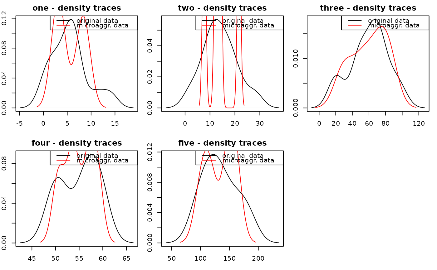 data(free1)
free1 <- as.data.frame(free1)
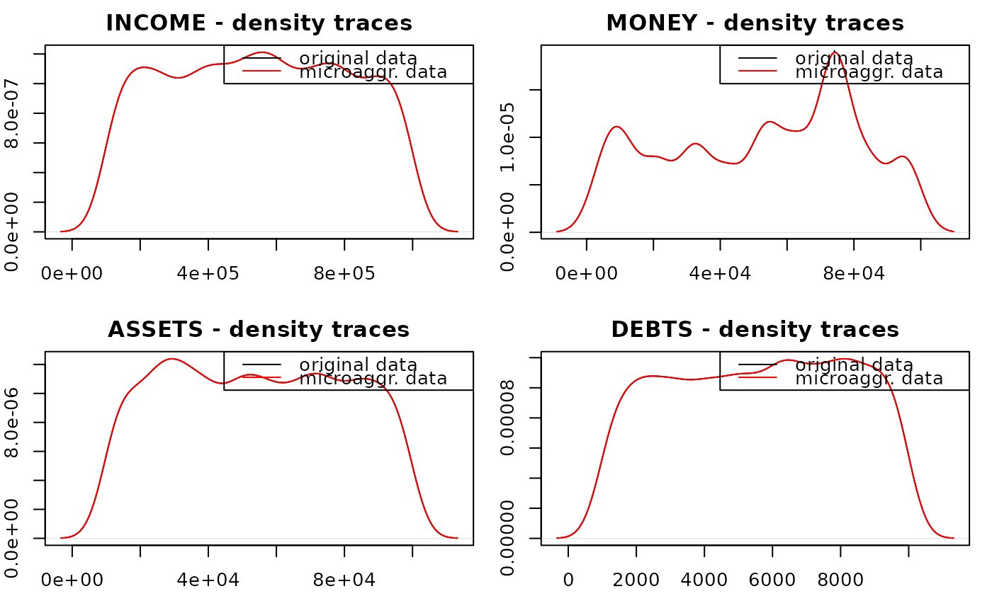
plotMicro(
x = microaggregation(free1[,31:34], method = "onedims"),
p = 1,
which.plot = 1
)
data(free1)
free1 <- as.data.frame(free1)
plotMicro(
x = microaggregation(free1[,31:34], method = "onedims"),
p = 1,
which.plot = 1
)
 ## disclosure risk (interval) and data utility:
m1 <- microaggregation(Tarragona, method = "onedims", aggr = 3)
dRisk(obj = Tarragona, xm = m1$mx)
#> [1] 0.8717026
dRisk(obj = Tarragona, xm = m2$mx)
#> [1] 0.004796163
dUtility(obj = Tarragona, xm = m1$mx)
#> [1] 120.8887
dUtility(obj = Tarragona, xm = m2$mx)
#> [1] 1512.416
## Fast generation of synthetic data with approximately
## the same covariance matrix as the original one.
data(mtcars)
cov(mtcars[, 4:6])
#> hp drat wt
#> hp 4700.86694 -16.4511089 44.1926613
#> drat -16.45111 0.2858814 -0.3727207
#> wt 44.19266 -0.3727207 0.9573790
df_gen <- dataGen(obj = mtcars[, 4:6], n = 200)
cov(df_gen)
#> hp drat wt
#> hp 4540.18921 -16.4344451 44.3904027
#> drat -16.43445 0.2984788 -0.4078128
#> wt 44.39040 -0.4078128 0.9892510
pairs(mtcars[, 4:6])
## disclosure risk (interval) and data utility:
m1 <- microaggregation(Tarragona, method = "onedims", aggr = 3)
dRisk(obj = Tarragona, xm = m1$mx)
#> [1] 0.8717026
dRisk(obj = Tarragona, xm = m2$mx)
#> [1] 0.004796163
dUtility(obj = Tarragona, xm = m1$mx)
#> [1] 120.8887
dUtility(obj = Tarragona, xm = m2$mx)
#> [1] 1512.416
## Fast generation of synthetic data with approximately
## the same covariance matrix as the original one.
data(mtcars)
cov(mtcars[, 4:6])
#> hp drat wt
#> hp 4700.86694 -16.4511089 44.1926613
#> drat -16.45111 0.2858814 -0.3727207
#> wt 44.19266 -0.3727207 0.9573790
df_gen <- dataGen(obj = mtcars[, 4:6], n = 200)
cov(df_gen)
#> hp drat wt
#> hp 4540.18921 -16.4344451 44.3904027
#> drat -16.43445 0.2984788 -0.4078128
#> wt 44.39040 -0.4078128 0.9892510
pairs(mtcars[, 4:6])
 pairs(df_gen)
 ## Post-Randomization (PRAM)
x <- factor(sample(1:4, 250, replace = TRUE))
pr1 <- pram(x)
length(which(pr1$x_pram == x))
#> [1] 222
summary(pr1)
#> Variable: x
#>
#> ----------------------
#>
#> Frequencies in original and perturbed data:
#> x 1 2 3 4 NA
#> <char> <char> <char> <char> <char> <char>
#> 1: Original Frequencies 60 67 59 64 0
#> 2: Frequencies after Perturbation 55 68 65 62 0
#>
#> Transitions:
#> transition Frequency
#> <char> <int>
#> 1: 1 --> 1 52
#> 2: 1 --> 2 2
#> 3: 1 --> 3 3
#> 4: 1 --> 4 3
#> 5: 2 --> 1 2
#> 6: 2 --> 2 60
#> 7: 2 --> 3 4
#> 8: 2 --> 4 1
#> 9: 3 --> 1 1
#> 10: 3 --> 2 4
#> 11: 3 --> 3 53
#> 12: 3 --> 4 1
#> 13: 4 --> 2 2
#> 14: 4 --> 3 5
#> 15: 4 --> 4 57
#>
x2 <- factor(sample(1:4, 250, replace=TRUE))
length(which(pram(x2)$x_pram == x2))
#> [1] 234
data(free1)
marstat <- as.factor(free1[,"MARSTAT"])
marstatPramed <- pram(marstat)
summary(marstatPramed)
#> Variable: x
#>
#> ----------------------
#>
#> Frequencies in original and perturbed data:
#> x 1 2 3 4 NA
#> <char> <char> <char> <char> <char> <char>
#> 1: Original Frequencies 2547 162 171 1120 0
#> 2: Frequencies after Perturbation 2547 158 177 1118 0
#>
#> Transitions:
#> transition Frequency
#> <char> <int>
#> 1: 1 --> 1 2418
#> 2: 1 --> 2 28
#> 3: 1 --> 3 40
#> 4: 1 --> 4 61
#> 5: 2 --> 1 37
#> 6: 2 --> 2 120
#> 7: 2 --> 4 5
#> 8: 3 --> 1 30
#> 9: 3 --> 2 1
#> 10: 3 --> 3 134
#> 11: 3 --> 4 6
#> 12: 4 --> 1 62
#> 13: 4 --> 2 9
#> 14: 4 --> 3 3
#> 15: 4 --> 4 1046
#>
## The same functionality can be also applied to `sdcMicroObj`-objects
data(testdata)
## undo-functionality is by default restricted to data sets
## with <= `1e5` rows; to modify, env-var `sdcMicro_maxsize_undo`
## can to be changed before creating a problem instance
Sys.setenv("sdcMicro_maxsize_undo" = 1e6)
## create an object
testdata$water <- factor(testdata$water)
sdc <- createSdcObj(
dat = testdata,
keyVars = c("urbrur", "roof", "walls", "electcon", "water", "relat", "sex"),
numVars = c("expend", "income", "savings"),
w = "sampling_weight"
)
head(sdc@manipNumVars)
#> expend income savings
#> 1 90929693 57800000 116258.5
#> 2 27338058 25300000 279345.0
#> 3 26524717 69200000 5495381.0
#> 4 18073948 79600000 8695862.0
#> 5 6713247 90300000 203620.2
#> 6 49057636 32900000 1021268.0
## Display risk-measures
sdc@risk$global
#> $risk
#> [1] 0.00235334
#>
#> $risk_ER
#> [1] 10.7783
#>
#> $risk_pct
#> [1] 0.235334
#>
#> $threshold
#> [1] NA
#>
#> $max_risk
#> [1] 0.01
#>
sdc <- dRisk(sdc)
sdc@risk$numeric
#> [1] 1
## Generation of synthetic data
synthdat <- dataGen(sdc)
## use addNoise with default parameters (not suggested)
sdc <- addNoise(sdc, variables = c("expend", "income"))
head(sdc@manipNumVars)
#> expend income savings
#> 1 41361882 97867993 116258.5
#> 2 64827473 -26657240 279345.0
#> 3 31060570 43043526 5495381.0
#> 4 -9611113 -14374396 8695862.0
#> 5 28408470 124773683 203620.2
#> 6 26289579 -22533649 1021268.0
sdc@risk$numeric
#> [1] 0.00349345
## undolast step (remove adding noise)
sdc <- undolast(sdc)
head(sdc@manipNumVars)
#> expend income savings
#> 1 90929693 57800000 116258.5
#> 2 27338058 25300000 279345.0
#> 3 26524717 69200000 5495381.0
#> 4 18073948 79600000 8695862.0
#> 5 6713247 90300000 203620.2
#> 6 49057636 32900000 1021268.0
sdc@risk$numeric
#> [1] 1
## apply addNoise() with custom parameters
sdc <- addNoise(sdc, noise = 0.2)
head(sdc@manipNumVars)
#> expend income savings
#> 1 90879125 57708353 117704.0
#> 2 27236121 25375257 276831.9
#> 3 26524892 69188007 5489039.9
#> 4 18066834 79568690 8703730.8
#> 5 6619469 90342123 193098.3
#> 6 49075964 32868647 1025826.1
sdc@risk$numeric
#> [1] 1
## LocalSuppression
sdc <- undolast(sdc)
head(sdc@risk$individual)
#> risk fk Fk
#> [1,] 9.433072e-05 107 10700
#> [2,] 9.900010e-05 102 10200
#> [3,] 5.713959e-05 176 17600
#> [4,] 5.713959e-05 176 17600
#> [5,] 2.221729e-04 46 4600
#> [6,] 2.272211e-04 45 4500
sdc@risk$global
#> $risk
#> [1] 0.00235334
#>
#> $risk_ER
#> [1] 10.7783
#>
#> $risk_pct
#> [1] 0.235334
#>
#> $threshold
#> [1] NA
#>
#> $max_risk
#> [1] 0.01
#>
sdc <- localSuppression(sdc)
head(sdc@risk$individual)
#> risk fk Fk
#> [1,] 9.258402e-05 109 10900
#> [2,] 9.900010e-05 102 10200
#> [3,] 5.649398e-05 178 17800
#> [4,] 5.649398e-05 178 17800
#> [5,] 2.173441e-04 47 4700
#> [6,] 2.221729e-04 46 4600
sdc@risk$global
#> $risk
#> [1] 0.0006729827
#>
#> $risk_ER
#> [1] 3.082261
#>
#> $risk_pct
#> [1] 0.06729827
#>
#> $threshold
#> [1] NA
#>
#> $max_risk
#> [1] 0.01
#>
## microaggregation
sdc <- undolast(sdc)
head(get.sdcMicroObj(sdc, type = "manipNumVars"))
#> expend income savings
#> 1 90929693 57800000 116258.5
#> 2 27338058 25300000 279345.0
#> 3 26524717 69200000 5495381.0
#> 4 18073948 79600000 8695862.0
#> 5 6713247 90300000 203620.2
#> 6 49057636 32900000 1021268.0
sdc <- microaggregation(sdc)
head(get.sdcMicroObj(sdc, type = "manipNumVars"))
#> expend income savings
#> 1 89216447 56066667 198935.2
#> 2 26627836 25933333 478764.1
#> 3 23178458 67700000 5579820.3
#> 4 16100539 81433333 8634904.7
#> 5 9097752 88200000 282854.7
#> 6 49866768 34400000 955027.8
## Post-Randomization
sdc <- undolast(sdc)
head(sdc@risk$individual)
#> risk fk Fk
#> [1,] 9.433072e-05 107 10700
#> [2,] 9.900010e-05 102 10200
#> [3,] 5.713959e-05 176 17600
#> [4,] 5.713959e-05 176 17600
#> [5,] 2.221729e-04 46 4600
#> [6,] 2.272211e-04 45 4500
sdc@risk$global
#> $risk
#> [1] 0.00235334
#>
#> $risk_ER
#> [1] 10.7783
#>
#> $risk_pct
#> [1] 0.235334
#>
#> $threshold
#> [1] NA
#>
#> $max_risk
#> [1] 0.01
#>
sdc <- pram(sdc, variables = "water")
#> Warning: If pram is applied on key variables, the k-anonymity and risk assessment are not useful anymore.
head(sdc@risk$individual)
#> risk fk Fk
#> [1,] 9.090083e-05 111 11100
#> [2,] 1.020304e-04 99 9900
#> [3,] 5.524557e-05 182 18200
#> [4,] 5.524557e-05 182 18200
#> [5,] 2.173441e-04 47 4700
#> [6,] 2.325041e-04 44 4400
sdc@risk$global
#> $risk
#> [1] 0.002744458
#>
#> $risk_ER
#> [1] 12.56962
#>
#> $risk_pct
#> [1] 0.2744458
#>
#> $threshold
#> [1] NA
#>
#> $max_risk
#> [1] 0.01
#>
## rankSwap
sdc <- undolast(sdc)
head(sdc@risk$individual)
#> risk fk Fk
#> [1,] 9.433072e-05 107 10700
#> [2,] 9.900010e-05 102 10200
#> [3,] 5.713959e-05 176 17600
#> [4,] 5.713959e-05 176 17600
#> [5,] 2.221729e-04 46 4600
#> [6,] 2.272211e-04 45 4500
sdc@risk$global
#> $risk
#> [1] 0.00235334
#>
#> $risk_ER
#> [1] 10.7783
#>
#> $risk_pct
#> [1] 0.235334
#>
#> $threshold
#> [1] NA
#>
#> $max_risk
#> [1] 0.01
#>
head(get.sdcMicroObj(sdc, type = "manipNumVars"))
#> expend income savings
#> 1 90929693 57800000 116258.5
#> 2 27338058 25300000 279345.0
#> 3 26524717 69200000 5495381.0
#> 4 18073948 79600000 8695862.0
#> 5 6713247 90300000 203620.2
#> 6 49057636 32900000 1021268.0
sdc <- rankSwap(sdc)
#> setting parameter R0 = 0.95 as no inputs have been specified.
head(get.sdcMicroObj(sdc, type = "manipNumVars"))
#> expend income savings
#> 1 86610132 61500000 231542.6
#> 2 31325662 21100000 231542.6
#> 3 31683630 71700000 5301221.0
#> 4 10950378 86900000 9323581.0
#> 5 8280068 93800000 231542.6
#> 6 56197900 26100000 1666254.0
head(sdc@risk$individual)
#> risk fk Fk
#> [1,] 9.433072e-05 107 10700
#> [2,] 9.900010e-05 102 10200
#> [3,] 5.713959e-05 176 17600
#> [4,] 5.713959e-05 176 17600
#> [5,] 2.221729e-04 46 4600
#> [6,] 2.272211e-04 45 4500
sdc@risk$global
#> $risk
#> [1] 0.00235334
#>
#> $risk_ER
#> [1] 10.7783
#>
#> $risk_pct
#> [1] 0.235334
#>
#> $threshold
#> [1] NA
#>
#> $max_risk
#> [1] 0.01
#>
## topBotCoding
head(get.sdcMicroObj(sdc, type = "manipNumVars"))
#> expend income savings
#> 1 86610132 61500000 231542.6
#> 2 31325662 21100000 231542.6
#> 3 31683630 71700000 5301221.0
#> 4 10950378 86900000 9323581.0
#> 5 8280068 93800000 231542.6
#> 6 56197900 26100000 1666254.0
sdc@risk$numeric
#> [1] 0.008078603
sdc <- topBotCoding(
obj = sdc,
value = 60000000,
replacement = 62000000,
column = "income"
)
head(get.sdcMicroObj(sdc, type = "manipNumVars"))
#> expend income savings
#> 1 86610132 62000000 231542.6
#> 2 31325662 21100000 231542.6
#> 3 31683630 62000000 5301221.0
#> 4 10950378 62000000 9323581.0
#> 5 8280068 62000000 231542.6
#> 6 56197900 26100000 1666254.0
sdc@risk$numeric
#> [1] 0.00371179
## LocalRecProg
data(testdata2)
keyVars <- c("urbrur", "roof", "walls", "water", "sex")
w <- "sampling_weight"
sdc <- createSdcObj(testdata2,
keyVars = keyVars,
weightVar = w
)
sdc@risk$global
#> $risk
#> [1] 0.04651687
#>
#> $risk_ER
#> [1] 4.326069
#>
#> $risk_pct
#> [1] 4.651687
#>
#> $threshold
#> [1] 0
#>
#> $max_risk
#> [1] 0.01
#>
sdc <- LocalRecProg(sdc)
sdc@risk$global
#> $risk
#> [1] 0.003713992
#>
#> $risk_ER
#> [1] 0.3454013
#>
#> $risk_pct
#> [1] 0.3713992
#>
#> $threshold
#> [1] NA
#>
#> $max_risk
#> [1] 0.01
#>
## Model-based risks using a formula
form <- as.formula(paste("~", paste(keyVars, collapse = "+")))
sdc <- modRisk(sdc, method = "default", formulaM = form)
#> Warning: glm.fit: algorithm did not converge
#> Warning: glm.fit: fitted rates numerically 0 occurred
get.sdcMicroObj(sdc, "risk")$model
#> The estimated model (using method 'default') was:
#> ~ urbrur + roof + walls + water + sex
#> global risk-measures:
#> Risk-Measure 1: 0.372 (37.158 %)
#> Risk-Measure 2: 0.635 (63.477 %)
sdc <- modRisk(sdc, method = "CE", formulaM = form)
#> Warning: glm.fit: algorithm did not converge
#> Warning: glm.fit: fitted rates numerically 0 occurred
get.sdcMicroObj(sdc, "risk")$model
#> The estimated model (using method 'CE') was:
#> ~ urbrur + roof + walls + water + sex
#> global risk-measures:
#> Risk-Measure 1: 0.372 (37.158 %)
#> Risk-Measure 2: 0.635 (63.477 %)
sdc <- modRisk(sdc, method = "PML", formulaM = form)
#> Warning: glm.fit: algorithm did not converge
#> Warning: glm.fit: fitted rates numerically 0 occurred
get.sdcMicroObj(sdc, "risk")$model
#> The estimated model (using method 'PML') was:
#> ~ urbrur + roof + walls + water + sex
#> global risk-measures:
#> Risk-Measure 1: 0.372 (37.158 %)
#> Risk-Measure 2: 0.635 (63.477 %)
sdc <- modRisk(sdc, method = "weightedLLM", formulaM = form)
#> Warning: glm.fit: algorithm did not converge
get.sdcMicroObj(sdc, "risk")$model
#> The estimated model (using method 'weightedLLM') was:
#> ~ urbrur + roof + walls + water + sex
#> global risk-measures:
#> Risk-Measure 1: 0.372 (37.158 %)
#> Risk-Measure 2: 0.635 (63.477 %)
sdc <- modRisk(sdc, method = "IPF", formulaM = form)
get.sdcMicroObj(sdc, "risk")$model
#> The estimated model (using method 'IPF') was:
#> ~ urbrur + roof + walls + water + sex
#> global risk-measures:
#> Risk-Measure 1: 0.372 (37.158 %)
#> Risk-Measure 2: 0.635 (63.477 %)
# }
## Post-Randomization (PRAM)
x <- factor(sample(1:4, 250, replace = TRUE))
pr1 <- pram(x)
length(which(pr1$x_pram == x))
#> [1] 222
summary(pr1)
#> Variable: x
#>
#> ----------------------
#>
#> Frequencies in original and perturbed data:
#> x 1 2 3 4 NA
#> <char> <char> <char> <char> <char> <char>
#> 1: Original Frequencies 60 67 59 64 0
#> 2: Frequencies after Perturbation 55 68 65 62 0
#>
#> Transitions:
#> transition Frequency
#> <char> <int>
#> 1: 1 --> 1 52
#> 2: 1 --> 2 2
#> 3: 1 --> 3 3
#> 4: 1 --> 4 3
#> 5: 2 --> 1 2
#> 6: 2 --> 2 60
#> 7: 2 --> 3 4
#> 8: 2 --> 4 1
#> 9: 3 --> 1 1
#> 10: 3 --> 2 4
#> 11: 3 --> 3 53
#> 12: 3 --> 4 1
#> 13: 4 --> 2 2
#> 14: 4 --> 3 5
#> 15: 4 --> 4 57
#>
x2 <- factor(sample(1:4, 250, replace=TRUE))
length(which(pram(x2)$x_pram == x2))
#> [1] 234
data(free1)
marstat <- as.factor(free1[,"MARSTAT"])
marstatPramed <- pram(marstat)
summary(marstatPramed)
#> Variable: x
#>
#> ----------------------
#>
#> Frequencies in original and perturbed data:
#> x 1 2 3 4 NA
#> <char> <char> <char> <char> <char> <char>
#> 1: Original Frequencies 2547 162 171 1120 0
#> 2: Frequencies after Perturbation 2547 158 177 1118 0
#>
#> Transitions:
#> transition Frequency
#> <char> <int>
#> 1: 1 --> 1 2418
#> 2: 1 --> 2 28
#> 3: 1 --> 3 40
#> 4: 1 --> 4 61
#> 5: 2 --> 1 37
#> 6: 2 --> 2 120
#> 7: 2 --> 4 5
#> 8: 3 --> 1 30
#> 9: 3 --> 2 1
#> 10: 3 --> 3 134
#> 11: 3 --> 4 6
#> 12: 4 --> 1 62
#> 13: 4 --> 2 9
#> 14: 4 --> 3 3
#> 15: 4 --> 4 1046
#>
## The same functionality can be also applied to `sdcMicroObj`-objects
data(testdata)
## undo-functionality is by default restricted to data sets
## with <= `1e5` rows; to modify, env-var `sdcMicro_maxsize_undo`
## can to be changed before creating a problem instance
Sys.setenv("sdcMicro_maxsize_undo" = 1e6)
## create an object
testdata$water <- factor(testdata$water)
sdc <- createSdcObj(
dat = testdata,
keyVars = c("urbrur", "roof", "walls", "electcon", "water", "relat", "sex"),
numVars = c("expend", "income", "savings"),
w = "sampling_weight"
)
head(sdc@manipNumVars)
#> expend income savings
#> 1 90929693 57800000 116258.5
#> 2 27338058 25300000 279345.0
#> 3 26524717 69200000 5495381.0
#> 4 18073948 79600000 8695862.0
#> 5 6713247 90300000 203620.2
#> 6 49057636 32900000 1021268.0
## Display risk-measures
sdc@risk$global
#> $risk
#> [1] 0.00235334
#>
#> $risk_ER
#> [1] 10.7783
#>
#> $risk_pct
#> [1] 0.235334
#>
#> $threshold
#> [1] NA
#>
#> $max_risk
#> [1] 0.01
#>
sdc <- dRisk(sdc)
sdc@risk$numeric
#> [1] 1
## Generation of synthetic data
synthdat <- dataGen(sdc)
## use addNoise with default parameters (not suggested)
sdc <- addNoise(sdc, variables = c("expend", "income"))
head(sdc@manipNumVars)
#> expend income savings
#> 1 41361882 97867993 116258.5
#> 2 64827473 -26657240 279345.0
#> 3 31060570 43043526 5495381.0
#> 4 -9611113 -14374396 8695862.0
#> 5 28408470 124773683 203620.2
#> 6 26289579 -22533649 1021268.0
sdc@risk$numeric
#> [1] 0.00349345
## undolast step (remove adding noise)
sdc <- undolast(sdc)
head(sdc@manipNumVars)
#> expend income savings
#> 1 90929693 57800000 116258.5
#> 2 27338058 25300000 279345.0
#> 3 26524717 69200000 5495381.0
#> 4 18073948 79600000 8695862.0
#> 5 6713247 90300000 203620.2
#> 6 49057636 32900000 1021268.0
sdc@risk$numeric
#> [1] 1
## apply addNoise() with custom parameters
sdc <- addNoise(sdc, noise = 0.2)
head(sdc@manipNumVars)
#> expend income savings
#> 1 90879125 57708353 117704.0
#> 2 27236121 25375257 276831.9
#> 3 26524892 69188007 5489039.9
#> 4 18066834 79568690 8703730.8
#> 5 6619469 90342123 193098.3
#> 6 49075964 32868647 1025826.1
sdc@risk$numeric
#> [1] 1
## LocalSuppression
sdc <- undolast(sdc)
head(sdc@risk$individual)
#> risk fk Fk
#> [1,] 9.433072e-05 107 10700
#> [2,] 9.900010e-05 102 10200
#> [3,] 5.713959e-05 176 17600
#> [4,] 5.713959e-05 176 17600
#> [5,] 2.221729e-04 46 4600
#> [6,] 2.272211e-04 45 4500
sdc@risk$global
#> $risk
#> [1] 0.00235334
#>
#> $risk_ER
#> [1] 10.7783
#>
#> $risk_pct
#> [1] 0.235334
#>
#> $threshold
#> [1] NA
#>
#> $max_risk
#> [1] 0.01
#>
sdc <- localSuppression(sdc)
head(sdc@risk$individual)
#> risk fk Fk
#> [1,] 9.258402e-05 109 10900
#> [2,] 9.900010e-05 102 10200
#> [3,] 5.649398e-05 178 17800
#> [4,] 5.649398e-05 178 17800
#> [5,] 2.173441e-04 47 4700
#> [6,] 2.221729e-04 46 4600
sdc@risk$global
#> $risk
#> [1] 0.0006729827
#>
#> $risk_ER
#> [1] 3.082261
#>
#> $risk_pct
#> [1] 0.06729827
#>
#> $threshold
#> [1] NA
#>
#> $max_risk
#> [1] 0.01
#>
## microaggregation
sdc <- undolast(sdc)
head(get.sdcMicroObj(sdc, type = "manipNumVars"))
#> expend income savings
#> 1 90929693 57800000 116258.5
#> 2 27338058 25300000 279345.0
#> 3 26524717 69200000 5495381.0
#> 4 18073948 79600000 8695862.0
#> 5 6713247 90300000 203620.2
#> 6 49057636 32900000 1021268.0
sdc <- microaggregation(sdc)
head(get.sdcMicroObj(sdc, type = "manipNumVars"))
#> expend income savings
#> 1 89216447 56066667 198935.2
#> 2 26627836 25933333 478764.1
#> 3 23178458 67700000 5579820.3
#> 4 16100539 81433333 8634904.7
#> 5 9097752 88200000 282854.7
#> 6 49866768 34400000 955027.8
## Post-Randomization
sdc <- undolast(sdc)
head(sdc@risk$individual)
#> risk fk Fk
#> [1,] 9.433072e-05 107 10700
#> [2,] 9.900010e-05 102 10200
#> [3,] 5.713959e-05 176 17600
#> [4,] 5.713959e-05 176 17600
#> [5,] 2.221729e-04 46 4600
#> [6,] 2.272211e-04 45 4500
sdc@risk$global
#> $risk
#> [1] 0.00235334
#>
#> $risk_ER
#> [1] 10.7783
#>
#> $risk_pct
#> [1] 0.235334
#>
#> $threshold
#> [1] NA
#>
#> $max_risk
#> [1] 0.01
#>
sdc <- pram(sdc, variables = "water")
#> Warning: If pram is applied on key variables, the k-anonymity and risk assessment are not useful anymore.
head(sdc@risk$individual)
#> risk fk Fk
#> [1,] 9.090083e-05 111 11100
#> [2,] 1.020304e-04 99 9900
#> [3,] 5.524557e-05 182 18200
#> [4,] 5.524557e-05 182 18200
#> [5,] 2.173441e-04 47 4700
#> [6,] 2.325041e-04 44 4400
sdc@risk$global
#> $risk
#> [1] 0.002744458
#>
#> $risk_ER
#> [1] 12.56962
#>
#> $risk_pct
#> [1] 0.2744458
#>
#> $threshold
#> [1] NA
#>
#> $max_risk
#> [1] 0.01
#>
## rankSwap
sdc <- undolast(sdc)
head(sdc@risk$individual)
#> risk fk Fk
#> [1,] 9.433072e-05 107 10700
#> [2,] 9.900010e-05 102 10200
#> [3,] 5.713959e-05 176 17600
#> [4,] 5.713959e-05 176 17600
#> [5,] 2.221729e-04 46 4600
#> [6,] 2.272211e-04 45 4500
sdc@risk$global
#> $risk
#> [1] 0.00235334
#>
#> $risk_ER
#> [1] 10.7783
#>
#> $risk_pct
#> [1] 0.235334
#>
#> $threshold
#> [1] NA
#>
#> $max_risk
#> [1] 0.01
#>
head(get.sdcMicroObj(sdc, type = "manipNumVars"))
#> expend income savings
#> 1 90929693 57800000 116258.5
#> 2 27338058 25300000 279345.0
#> 3 26524717 69200000 5495381.0
#> 4 18073948 79600000 8695862.0
#> 5 6713247 90300000 203620.2
#> 6 49057636 32900000 1021268.0
sdc <- rankSwap(sdc)
#> setting parameter R0 = 0.95 as no inputs have been specified.
head(get.sdcMicroObj(sdc, type = "manipNumVars"))
#> expend income savings
#> 1 86610132 61500000 231542.6
#> 2 31325662 21100000 231542.6
#> 3 31683630 71700000 5301221.0
#> 4 10950378 86900000 9323581.0
#> 5 8280068 93800000 231542.6
#> 6 56197900 26100000 1666254.0
head(sdc@risk$individual)
#> risk fk Fk
#> [1,] 9.433072e-05 107 10700
#> [2,] 9.900010e-05 102 10200
#> [3,] 5.713959e-05 176 17600
#> [4,] 5.713959e-05 176 17600
#> [5,] 2.221729e-04 46 4600
#> [6,] 2.272211e-04 45 4500
sdc@risk$global
#> $risk
#> [1] 0.00235334
#>
#> $risk_ER
#> [1] 10.7783
#>
#> $risk_pct
#> [1] 0.235334
#>
#> $threshold
#> [1] NA
#>
#> $max_risk
#> [1] 0.01
#>
## topBotCoding
head(get.sdcMicroObj(sdc, type = "manipNumVars"))
#> expend income savings
#> 1 86610132 61500000 231542.6
#> 2 31325662 21100000 231542.6
#> 3 31683630 71700000 5301221.0
#> 4 10950378 86900000 9323581.0
#> 5 8280068 93800000 231542.6
#> 6 56197900 26100000 1666254.0
sdc@risk$numeric
#> [1] 0.008078603
sdc <- topBotCoding(
obj = sdc,
value = 60000000,
replacement = 62000000,
column = "income"
)
head(get.sdcMicroObj(sdc, type = "manipNumVars"))
#> expend income savings
#> 1 86610132 62000000 231542.6
#> 2 31325662 21100000 231542.6
#> 3 31683630 62000000 5301221.0
#> 4 10950378 62000000 9323581.0
#> 5 8280068 62000000 231542.6
#> 6 56197900 26100000 1666254.0
sdc@risk$numeric
#> [1] 0.00371179
## LocalRecProg
data(testdata2)
keyVars <- c("urbrur", "roof", "walls", "water", "sex")
w <- "sampling_weight"
sdc <- createSdcObj(testdata2,
keyVars = keyVars,
weightVar = w
)
sdc@risk$global
#> $risk
#> [1] 0.04651687
#>
#> $risk_ER
#> [1] 4.326069
#>
#> $risk_pct
#> [1] 4.651687
#>
#> $threshold
#> [1] 0
#>
#> $max_risk
#> [1] 0.01
#>
sdc <- LocalRecProg(sdc)
sdc@risk$global
#> $risk
#> [1] 0.003713992
#>
#> $risk_ER
#> [1] 0.3454013
#>
#> $risk_pct
#> [1] 0.3713992
#>
#> $threshold
#> [1] NA
#>
#> $max_risk
#> [1] 0.01
#>
## Model-based risks using a formula
form <- as.formula(paste("~", paste(keyVars, collapse = "+")))
sdc <- modRisk(sdc, method = "default", formulaM = form)
#> Warning: glm.fit: algorithm did not converge
#> Warning: glm.fit: fitted rates numerically 0 occurred
get.sdcMicroObj(sdc, "risk")$model
#> The estimated model (using method 'default') was:
#> ~ urbrur + roof + walls + water + sex
#> global risk-measures:
#> Risk-Measure 1: 0.372 (37.158 %)
#> Risk-Measure 2: 0.635 (63.477 %)
sdc <- modRisk(sdc, method = "CE", formulaM = form)
#> Warning: glm.fit: algorithm did not converge
#> Warning: glm.fit: fitted rates numerically 0 occurred
get.sdcMicroObj(sdc, "risk")$model
#> The estimated model (using method 'CE') was:
#> ~ urbrur + roof + walls + water + sex
#> global risk-measures:
#> Risk-Measure 1: 0.372 (37.158 %)
#> Risk-Measure 2: 0.635 (63.477 %)
sdc <- modRisk(sdc, method = "PML", formulaM = form)
#> Warning: glm.fit: algorithm did not converge
#> Warning: glm.fit: fitted rates numerically 0 occurred
get.sdcMicroObj(sdc, "risk")$model
#> The estimated model (using method 'PML') was:
#> ~ urbrur + roof + walls + water + sex
#> global risk-measures:
#> Risk-Measure 1: 0.372 (37.158 %)
#> Risk-Measure 2: 0.635 (63.477 %)
sdc <- modRisk(sdc, method = "weightedLLM", formulaM = form)
#> Warning: glm.fit: algorithm did not converge
get.sdcMicroObj(sdc, "risk")$model
#> The estimated model (using method 'weightedLLM') was:
#> ~ urbrur + roof + walls + water + sex
#> global risk-measures:
#> Risk-Measure 1: 0.372 (37.158 %)
#> Risk-Measure 2: 0.635 (63.477 %)
sdc <- modRisk(sdc, method = "IPF", formulaM = form)
get.sdcMicroObj(sdc, "risk")$model
#> The estimated model (using method 'IPF') was:
#> ~ urbrur + roof + walls + water + sex
#> global risk-measures:
#> Risk-Measure 1: 0.372 (37.158 %)
#> Risk-Measure 2: 0.635 (63.477 %)
# }